Leonardo Capitani
  • Home
  • Research Projects
  • Learning
  • Open Science
  • Science Communication
  • Consulting
  • Contact
  1. Ecological Modelling
  2. Ecopath with Ecosim (Rpath)
  • All notebooks
  • Open Science
    • Registered Reports: what are they?
  • Ecological Modelling
    • Empirical Dynamic Modelling: intro
    • Convergent Cross Mapping
    • Gaussian Processes
    • Ecopath with Ecosim (Rpath)
  • Statistics
    • Priors
    • Measurement Error
    • Sample Size Planning

On this page

  • Why this notebook
  • Part 1 — What Ecopath is
  • Part 2 — Rpath
  • Part 3 — Rebuilding the Rocas Atoll model
    • Two data problems worth naming
    • Does the rebuild reproduce the published model?
    • Balancing
  • Part 4 — Ecosim under warming
    • The temperature forcing
    • Is the baseline stationary?
    • Results
    • Where the model stops being believable
  • What to take from this
  • References
  1. Ecological Modelling
  2. Ecopath with Ecosim (Rpath)

Ecopath with Ecosim, and its R counterpart Rpath

  • Show All Code
  • Hide All Code

  • View Source
Author

Leonardo Capitani

Published

August 11, 2026

Modified

August 11, 2026

Why this notebook

Ecopath with Ecosim (EwE) is the most widely used food-web modelling framework in fisheries and marine ecology, and for most of its life it has been used through a Windows GUI. That is a problem for reproducibility: a model built by clicking is hard to version, hard to review, and hard to rerun.

Rpath is an R implementation of the same equations. This notebook introduces the framework, then rebuilds a real published model — the Rocas Atoll food web from Capitani et al. 2022 — entirely in code, and runs it forward under warming scenarios. I am the first author of that paper, so I am rebuilding my own model here, which also makes this an honest test of whether my own archived inputs are complete enough to reconstruct it.

Part 1 — What Ecopath is

Ecopath is a mass-balance snapshot of a food web. It assumes that, over the period described, production of each group is accounted for by everything that removes it. The framework goes back to Polovina (1984) and was developed into its modern form by Christensen and Pauly (1992) and Christensen and Walters (2004).

The first master equation says production is either eaten, caught, exported, or accumulated:

\[ B_i \cdot \left(\frac{P}{B}\right)_i \cdot EE_i \;=\; \sum_{j} B_j \cdot \left(\frac{Q}{B}\right)_j \cdot DC_{ji} \;+\; Y_i \;+\; E_i \;+\; BA_i \]

where \(B\) is biomass, \(P/B\) production per unit biomass (equal to total mortality \(Z\) under steady state), \(Q/B\) consumption per unit biomass, \(DC_{ji}\) the fraction of prey \(i\) in predator \(j\)’s diet, \(Y\) the fishery catch, \(E\) net migration, \(BA\) biomass accumulation, and \(EE\) the ecotrophic efficiency — the fraction of production used inside the system.

The second is an energy balance for each consumer:

\[ Q_i \;=\; P_i \;+\; R_i \;+\; U_i \]

consumption equals production plus respiration plus unassimilated food.

The practical consequence is what makes Ecopath useful: for every group you supply three of the four quantities \(B\), \(P/B\), \(Q/B\), \(EE\), and the model solves for the fourth. EE is the one that is hardest to measure and easiest to leave for the model to estimate.

ImportantThe balance criterion

A model is balanced when \(EE \le 1\) for every group. \(EE > 1\) means the food web demands more of a group than it can produce — the model is asking a prey population to be eaten more than once. Getting from an unbalanced first draft to a balanced model is most of the work in any EwE study.

Ecosim (Walters et al. 1997) makes the snapshot dynamic. It re-expresses the same web as coupled differential equations,

\[ \frac{dB_i}{dt} \;=\; g_i \sum_j Q_{ji} \;-\; \sum_j Q_{ij} \;+\; I_i \;-\; (M0_i + F_i + e_i)\,B_i \]

with \(g_i\) the growth efficiency, and predation rates set by foraging arena theory: prey are split into a vulnerable and an invulnerable pool, and the exchange rate between them (the vulnerability, \(v\)) decides whether a predator–prey link is top-down (\(v\) large) or bottom-up (\(v\) near 1) controlled. Vulnerabilities are the main tuning parameters when fitting Ecosim to time series.

Part 2 — Rpath

Rpath is the R implementation, developed at NOAA’s Ecosystem Dynamics and Assessment Branch. It reproduces the Ecopath algorithm and the Ecosim differential equations in C++ under an R interface, and it is the reference for reproducible EwE work (Lucey et al. 2020).

Authors of the package — Kerim Aydin, Sean Lucey, Sarah Gaichas, Sarah Weisberg and Andy Whitehouse, with contributions from Bia Dias, Ron Klasky, Andy Beet and Max Grezlik (Aydin et al. 2026). The package documentation and vignette are at noaa-edab.github.io/Rpath.

Code
library(Rpath)
library(data.table)
library(ggplot2)

cat("Rpath version:", as.character(packageVersion("Rpath")), "\n")
Rpath version: 1.1.0 

The workflow has three objects: a parameter object (create.rpath.params), a balanced model (rpath), and a scenario (rsim.scenario) that you run forward with rsim.run.

Part 3 — Rebuilding the Rocas Atoll model

Rocas Atoll is the only atoll in the South Atlantic, a fully protected no-take reserve off north-eastern Brazil. The published model has 28 functional groups: 16 fish groups, sea birds, turtles, cephalopods, lobsters, two benthic invertebrate groups, corals, zooplankton, phytoplankton, two algal groups, and detritus.

Figure 2 of the paper shows the whole web, in the balanced 2012 state and under the warmest 2100 projection:
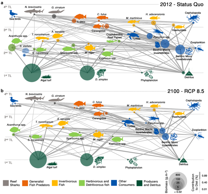
Figure 1: The Rocas Atoll food web as modelled. Node size is biomass, link thickness is the contribution to diet, vertical position is trophic level. a) the balanced 2012 model; b) the projected 2100 state under RCP 8.5. Figure 2 from Capitani et al. 2022, Ecosystems, reproduced here by the first author.

The inputs below come from the archived model in my repository Atoll_Rocas_project: the basic estimates and diet matrix that the published Ecopath model was built from.

Code
D <- "data/"
basic <- fread(paste0(D, "rocas_basic_input.csv"))
diet  <- fread(paste0(D, "rocas_diet.csv"))

knitr::kable(
  basic[, .(Group, Type, `B (t/km2)` = round(Biomass, 3),
            `P/B (/yr)` = PB, `Q/B (/yr)` = QB,
            `EE published` = round(EE_published, 3),
            `BA (t/km2/yr)` = round(BioAcc, 3))],
  caption = "Basic inputs of the published Rocas Atoll model. Type 0 = consumer, 1 = producer, 2 = detritus."
)
Basic inputs of the published Rocas Atoll model. Type 0 = consumer, 1 = producer, 2 = detritus.
Group Type B (t/km2) P/B (/yr) Q/B (/yr) EE published BA (t/km2/yr)
Sea birds 0 0.020 5.400 80.00 0.000 0.000
Negaprion brevirostris 0 0.170 0.228 3.70 0.000 0.000
Ginglymostoma cirratum 0 1.800 0.217 3.60 0.820 0.320
Lutjanus jocu 0 2.220 0.522 6.30 0.005 0.000
Cephalopholis fulva 0 0.200 0.650 5.51 0.948 0.060
Carangidae 0 2.120 0.618 13.20 0.602 0.636
Acanthurus spp. 0 9.860 0.828 12.90 0.278 -0.246
Stegastes rocasensis 0 0.460 1.250 17.10 0.675 0.028
Thalassoma noronhanum 0 0.200 1.192 16.40 0.789 -0.005
Abudefduf saxatilis 0 0.990 0.892 13.00 0.451 -0.050
Sparisoma spp. 0 1.130 0.648 7.20 0.197 0.113
Melichthys niger 0 0.270 0.764 11.60 0.515 0.081
Kyphosus spp. 0 0.460 0.621 24.40 0.111 0.000
Mulloidichthys martinicus 0 0.416 0.719 11.10 0.601 0.166
Holocentrus adscensionis 0 2.118 0.750 8.30 0.977 0.593
Haemulidae 0 0.962 0.792 11.60 0.837 0.125
Small omnivore fish 0 0.790 1.870 10.57 0.265 -0.237
Turtles 0 0.022 0.290 2.35 0.000 0.000
Cephalopoda 0 0.405 6.400 36.50 0.948 0.000
Panulirus spp. 0 5.100 1.280 7.40 0.357 0.000
Benthic macroinvertebrates 0 16.704 3.800 10.00 0.900 0.000
Benthic microinvertebrates 0 25.690 4.940 16.69 0.850 0.000
Siderastrea stellata 0 0.711 1.660 9.40 0.000 0.000
Zooplankton 0 0.238 87.000 160.00 0.935 0.000
Phytoplankton 1 0.130 109.500 NA 0.701 0.000
Digenea simplex 1 211.638 274.000 NA 0.001 0.000
Other algal turf 1 802.312 323.000 NA 0.000 0.000
Detritus 2 1.000 NA NA 0.002 0.000

Two data problems worth naming

Rebuilding an archived model is never a clean copy, and this one is a good illustration of why:

  1. The archived diet matrix is rounded to two decimals, so predator columns sum to 0.99 or 1.05 rather than 1. Rpath requires columns summing to exactly 1, so each column is renormalised.
  2. The zooplankton column is incomplete in the archived CSV (it sums to 0.4 and shows zooplankton eating itself). The source spreadsheet gives the intended diet — 0.4 phytoplankton, 0.6 detritus — which is what I use.

A third trap is subtler: group 17 is called “Cryptobenthic reef fishes” in the diet file but “Small omnivore fish” in the basic-input file. Joining the two tables by name silently drops every predation link on that group and produces a negative ecotrophic efficiency. Joining by group number is the fix. This is the kind of error that is invisible unless you check the output against the published values, which is exactly what we do below.

Code
build_rocas <- function(B_thal = 0.20, B_phyto = 0.13, zero_BA = FALSE,
                        export_algae = FALSE) {

  basic <- fread(paste0(D, "rocas_basic_input.csv"))
  diet  <- fread(paste0(D, "rocas_diet.csv"))
  basic[Group == "Thalassoma noronhanum", Biomass := B_thal]
  basic[Group == "Phytoplankton",         Biomass := B_phyto]
  if (isTRUE(zero_BA)) basic[, BioAcc := 0]

  groups <- basic$Group; types <- basic$Type

  # prey rows identified by GROUP NUMBER, not by name (see note above)
  dm <- as.matrix(diet[, 3:26]); dm[is.na(dm)] <- 0
  rownames(dm) <- c(groups, "Import")
  colnames(dm) <- groups[1:24]

  dm[, "Zooplankton"] <- 0
  dm["Phytoplankton", "Zooplankton"] <- 0.4
  dm["Detritus",      "Zooplankton"] <- 0.6
  dm <- sweep(dm, 2, colSums(dm), "/")          # published table is rounded

  # Rocas is a no-take reserve, but Rpath requires >= 1 fleet: add a zero-catch one
  p <- create.rpath.params(group = c(groups, "No-take reserve"),
                           type  = c(types, 3))
  pad <- function(x, fill = NA) c(x, fill)
  p$model[, Biomass  := pad(basic$Biomass)]
  p$model[, PB       := pad(basic$PB)]
  p$model[, QB       := pad(ifelse(basic$Type == 0, basic$QB, NA))]
  p$model[, EE       := NA_real_]
  p$model[, ProdCons := NA_real_]
  p$model[, BioAcc   := pad(ifelse(basic$Type == 2, NA, basic$BioAcc))]
  p$model[, Unassim  := pad(ifelse(basic$Type == 0, 0.2, 0))]
  p$model[, Detritus := pad(ifelse(basic$Type == 2, 0, 1))]
  p$model[, `No-take reserve` := 0][, `No-take reserve.disc` := 0]
  p$model[Type == 3, `:=`(`No-take reserve` = NA, `No-take reserve.disc` = NA,
                          Detritus = 0)]
  if (isTRUE(export_algae))
    p$model[Group %in% c("Digenea simplex", "Other algal turf"), Detritus := 0]

  for (pred in colnames(dm)) p$diet[[pred]] <- dm[as.character(p$diet$Group), pred]
  p$diet[is.na(p$diet)] <- 0

  m <- rpath(p, eco.name = "Rocas Atoll")
  attr(m, "params") <- p
  m
}

rocas0 <- build_rocas()
cat("groups with EE > 1:", sum(rocas0$EE[1:28] > 1), "\n")
groups with EE > 1: 2 

Does the rebuild reproduce the published model?

The published model supplied \(B\), \(P/B\) and \(Q/B\) and let Ecopath estimate \(EE\). So the honest test is: feed Rpath the same three, and compare the \(EE\) it estimates against the published values.

Code
cmp <- data.table(Group = basic$Group,
                  Published = round(basic$EE_published, 3),
                  Rpath     = round(rocas0$EE[1:28], 3))
cmp[, Difference := round(Rpath - Published, 3)]

knitr::kable(cmp, caption = "Ecotrophic efficiency: published model vs this rebuild.")
Ecotrophic efficiency: published model vs this rebuild.
Group Published Rpath Difference
Sea birds 0.000 0.000 0.000
Negaprion brevirostris 0.000 0.000 0.000
Ginglymostoma cirratum 0.820 0.820 0.000
Lutjanus jocu 0.005 0.192 0.187
Cephalopholis fulva 0.948 0.950 0.002
Carangidae 0.602 0.600 -0.002
Acanthurus spp. 0.278 0.275 -0.003
Stegastes rocasensis 0.675 0.667 -0.008
Thalassoma noronhanum 0.789 1.340 0.551
Abudefduf saxatilis 0.451 0.432 -0.019
Sparisoma spp. 0.197 0.198 0.001
Melichthys niger 0.515 0.516 0.001
Kyphosus spp. 0.111 0.111 0.000
Mulloidichthys martinicus 0.601 0.599 -0.002
Holocentrus adscensionis 0.977 0.979 0.002
Haemulidae 0.837 0.849 0.012
Small omnivore fish 0.265 0.266 0.001
Turtles 0.000 0.996 0.996
Cephalopoda 0.948 0.892 -0.056
Panulirus spp. 0.357 0.347 -0.010
Benthic macroinvertebrates 0.900 0.899 -0.001
Benthic microinvertebrates 0.850 0.839 -0.011
Siderastrea stellata 0.000 0.000 0.000
Zooplankton 0.935 0.490 -0.445
Phytoplankton 0.701 1.234 0.533
Digenea simplex 0.001 0.001 0.000
Other algal turf 0.000 0.000 0.000
Detritus 0.002 0.002 0.000
Code
cat("groups matching within 0.02:", sum(abs(cmp$Difference) < 0.02), "of 28\n")
groups matching within 0.02: 22 of 28

Twenty-two of 28 groups reproduce to within 0.02. The six that do not are traceable to the two data problems above — the patched zooplankton column changes the predation on zooplankton and phytoplankton, and rounding in the diet matrix propagates into the groups with the tightest budgets. Two of them, Thalassoma noronhanum and phytoplankton, come out above 1, so this rebuild is not balanced as it stands.

Balancing

The classic Ecopath balancing move is to change the fewest inputs you can defend, and say which ones. Both offending groups need slightly more biomass than the rounded diet matrix implies, so I raise those two biomasses and leave the other 26 groups untouched.

Code
rocas <- build_rocas(B_thal = 0.30, B_phyto = 0.17)

cat("max EE:", round(max(rocas$EE[1:28]), 3),
    "| groups with EE > 1:", sum(rocas$EE[1:28] > 1), "\n")
max EE: 0.996 | groups with EE > 1: 0 
Code
knitr::kable(
  data.table(Group = basic$Group,
             `Trophic level` = round(rocas$TL[1:28], 2),
             `Biomass (t/km2)` = round(rocas$Biomass[1:28], 3),
             EE = round(rocas$EE[1:28], 3))[order(-`Trophic level`)][1:10],
  caption = "The ten highest trophic levels in the balanced rebuild."
)
The ten highest trophic levels in the balanced rebuild.
Group Trophic level Biomass (t/km2) EE
Negaprion brevirostris 3.56 0.170 0.000
Sea birds 3.47 0.020 0.000
Ginglymostoma cirratum 3.47 1.800 0.820
Lutjanus jocu 3.28 2.220 0.192
Cephalopholis fulva 3.27 0.200 0.950
Holocentrus adscensionis 3.19 2.118 0.979
Cephalopoda 3.19 0.405 0.892
Haemulidae 3.09 0.962 0.849
Mulloidichthys martinicus 3.07 0.416 0.599
Carangidae 3.02 2.120 0.600

The model is now balanced, and the trophic levels match the published ones closely: lemon sharks and nurse sharks at the top around TL 3.5, the herbivores just above 2, and the algae and detritus at 1.

Code
nodes <- data.table(Group = rocas$Group[1:28], TL = rocas$TL[1:28],
                    B = rocas$Biomass[1:28])[, x := seq_len(.N)]

dm <- as.matrix(attr(rocas, "params")$diet[, -1])
rownames(dm) <- as.character(attr(rocas, "params")$diet$Group)

links <- rbindlist(lapply(colnames(dm), function(pred) {
  v <- dm[, pred]; v <- v[v > 0.05 & names(v) != "Import"]
  if (!length(v)) return(NULL)
  data.table(prey = names(v), pred = pred, w = as.numeric(v))
}))
links <- merge(links, nodes[, .(prey = Group, x0 = x, y0 = TL)], by = "prey")
links <- merge(links, nodes[, .(pred = Group, x1 = x, y1 = TL)], by = "pred")

ggplot() +
  geom_segment(data = links, aes(x0, y0, xend = x1, yend = y1, linewidth = w),
               colour = "grey65", alpha = 0.5) +
  scale_linewidth(range = c(0.2, 1.6), guide = "none") +
  geom_point(data = nodes, aes(x, TL, size = B), colour = "#1d4ed8", alpha = 0.75) +
  scale_size_area(max_size = 13, trans = "sqrt", name = "Biomass (t/km2)") +
  ggrepel::geom_text_repel(data = nodes, aes(x, TL, label = Group),
                           size = 2.7, max.overlaps = 40) +
  labs(x = NULL, y = "Trophic level") +
  theme_minimal(base_size = 11) +
  theme(axis.text.x = element_blank(), panel.grid.minor = element_blank())
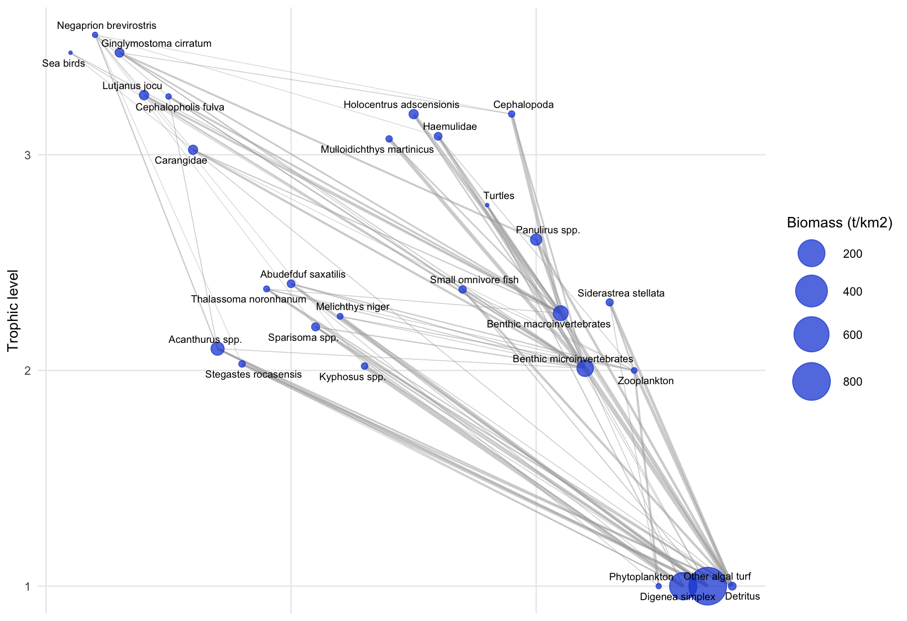
The balanced rebuild: every group at its estimated trophic level, sized by biomass, with diet links above 5% drawn. Compare with Figure 2a above.

Part 4 — Ecosim under warming

Two changes are needed before the model can be run forward.

Biomass accumulation is switched off. The Ecopath snapshot records non-zero \(BA\) for several groups, meaning the system was not in steady state in 2012. Carried into Ecosim, those trends compound for 89 years and the model runs away. A stationary baseline is the standard starting point for scenario work.

Unconsumed algal production is exported rather than sent to detritus. This is the interesting one. The two algal groups have very high turnover (\(P/B\) of 274 and 323 per year) and almost nothing eats them (\(EE < 0.001\)), so their unconsumed production is enormous — around \(2.6 \times 10^5\) t/km²/yr for turf alone. Ecopath does not mind, because the surplus simply leaves the system. Ecosim does mind: routed into a detritus pool of 1 t/km², it floods the pool, the detritivores explode on it, and the whole web follows. Routing that surplus out of the system instead — biologically, turf production washing off an oceanic atoll — gives a stable baseline.

WarningThe cost of that choice

Exporting the algal surplus removes the detritivores’ main documented food supply, so the detritus group’s own \(EE\) rises above 1 in the static solution. There is no configuration of this archived model that is simultaneously balanced in Ecopath and stationary in Ecosim; the published study fitted vulnerabilities to time series to get there, and that fitting is not fully in the archive. Everything below should therefore be read as relative to the unforced baseline, not as a reproduction of the published projections.

Code
rocas_sim <- build_rocas(B_thal = 0.30, B_phyto = 0.17,
                         zero_BA = TRUE, export_algae = TRUE)

The temperature forcing

Each group gets a thermal performance curve built from its observed thermal range — the 10th percentile, optimum, and 90th percentile of the temperatures at which it occurs, taken from the paper’s compilation. Performance is Gaussian around the optimum, scaled so that it halves at the 10th and 90th percentiles, and it multiplies the group’s search rate, so a group pushed past its optimum forages less effectively.

Code
therm <- fread(paste0(D, "rocas_thermal_ranges.csv"))
therm[, Species := fifelse(Species == "Benthic macroinvert.", "Benthic macroinvertebrates",
              fifelse(Species == "Benthic microinvert.", "Benthic microinvertebrates",
              fifelse(Species == "Cryptobenthic reef fishes", "Small omnivore fish",
              fifelse(Species == "Algal turf", "Other algal turf", Species))))]
tw <- dcast(therm, Species ~ class, value.var = "temperature")

thermal_mult <- function(Temp, opt, p10, p90) {
  sL <- pmax((opt - p10) / 1.1774, 0.5)   # 1.1774 sigma -> performance = 0.5
  sR <- pmax((p90 - opt) / 1.1774, 0.5)
  exp(-0.5 * ((Temp - opt) / ifelse(Temp < opt, sL, sR))^2)
}

sst <- fread(paste0(D, "rocas_sst_rcp.csv"))
setnames(sst, c("Year", "RCP2.6", "RCP4.5", "RCP8.5"))

knitr::kable(sst[Year %in% c(2012, 2050, 2100)],
             caption = "Projected sea surface temperature at Rocas Atoll (deg C).")
Projected sea surface temperature at Rocas Atoll (deg C).
Year RCP2.6 RCP4.5 RCP8.5
2012 27.32164 27.34236 27.19856
2050 27.78806 28.22839 28.46531
2100 27.79162 28.62535 30.48841
Code
run_scenario <- function(m, scen = NULL) {
  p <- attr(m, "params")
  s <- rsim.scenario(m, p, years = sst$Year)
  if (!is.null(scen)) {
    Tm <- rep(sst[[scen]], each = 12)
    for (g in tw$Species) {
      if (!g %in% colnames(s$forcing$ForcedSearch)) next
      row <- tw[Species == g]
      f <- thermal_mult(Tm, row$opti, row$perc10, row$perc90)
      f <- f / f[1]                                   # relative to 2012
      n <- nrow(s$forcing$ForcedSearch)
      s$forcing$ForcedSearch[, g] <- c(f, rep(tail(f, 1), n))[1:n]
    }
  }
  rsim.run(s, method = "RK4", years = sst$Year)
}

runs <- list(Baseline = run_scenario(rocas_sim, NULL))
for (sc in c("RCP2.6", "RCP4.5", "RCP8.5")) runs[[sc]] <- run_scenario(rocas_sim, sc)

Is the baseline stationary?

Before believing any scenario, check that the unforced run stays put. If the baseline drifts, every “effect” you measure is partly just drift.

Code
fish <- c("Negaprion brevirostris","Ginglymostoma cirratum","Lutjanus jocu",
          "Cephalopholis fulva","Carangidae","Acanthurus spp.","Stegastes rocasensis",
          "Thalassoma noronhanum","Abudefduf saxatilis","Sparisoma spp.",
          "Melichthys niger","Kyphosus spp.","Mulloidichthys martinicus",
          "Holocentrus adscensionis","Haemulidae","Small omnivore fish")

tot_fish <- function(r) rowSums(r$out_Biomass[, fish, drop = FALSE])
b0 <- tot_fish(runs$Baseline)

cat(sprintf("baseline total fish biomass: %.2f t/km2 (2012) -> %.2f t/km2 (2100), %+.1f%%\n",
            b0[1], tail(b0, 1), 100 * (tail(b0, 1) / b0[1] - 1)))
baseline total fish biomass: 24.27 t/km2 (2012) -> 24.12 t/km2 (2100), -0.6%

The unforced run moves by well under one percent over 89 years, so the baseline is stationary and anything we see under forcing is the forcing.

Results

Code
dt <- rbindlist(lapply(names(runs)[-1], function(sc) {
  data.table(Year = sst$Year[1] + (seq_along(b0) - 1) / 12,
             Scenario = sc,
             Relative = tot_fish(runs[[sc]]) / b0)
}))

ggplot(dt[Year <= 2100], aes(Year, Relative, colour = Scenario)) +
  geom_hline(yintercept = 1, linetype = 2, colour = "grey50") +
  geom_line(linewidth = 0.9) +
  scale_colour_manual(values = c("RCP2.6" = "#2c7fb8", "RCP4.5" = "#e6a419",
                                 "RCP8.5" = "#c0392b")) +
  scale_y_continuous(labels = scales::percent) +
  labs(y = "Total fish biomass\n(relative to baseline)", x = NULL) +
  theme_minimal(base_size = 12) +
  theme(legend.position = "bottom", legend.title = element_blank())
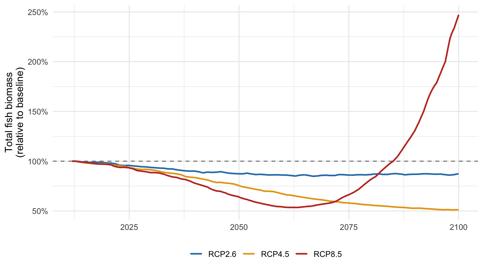
Total fish biomass under each warming scenario, relative to the unforced baseline in the same year.
Code
end <- length(b0)
res <- data.table(Scenario = names(runs)[-1],
                  `SST 2100 (deg C)` = round(unlist(sst[.N, .(RCP2.6, RCP4.5, RCP8.5)]), 2),
                  `Total fish vs baseline` =
                    sprintf("%+.1f%%", sapply(names(runs)[-1],
                            function(sc) 100 * (tot_fish(runs[[sc]])[end] / b0[end] - 1))))
knitr::kable(res, caption = "Total fish biomass in 2100 relative to the unforced baseline.")
Total fish biomass in 2100 relative to the unforced baseline.
Scenario SST 2100 (deg C) Total fish vs baseline
RCP2.6 27.79 -12.9%
RCP4.5 28.63 -49.0%
RCP8.5 30.49 +164.8%

Under RCP 2.6 the fish community loses around a tenth of its biomass, and under RCP 4.5 about half. The direction matches the published conclusion — warming simplifies this reef and takes biomass out of it — even though the magnitudes are not directly comparable, for the reasons in the warning above.

Where the model stops being believable

RCP 8.5 does not continue the pattern. It reports an increase, and the group-level results show why.

Code
ratio85 <- runs$RCP8.5$out_Biomass[end, fish] / runs$Baseline$out_Biomass[end, fish]
knitr::kable(data.table(Group = names(ratio85),
                        `x baseline in 2100` = round(as.numeric(ratio85), 3))[order(-`x baseline in 2100`)],
             caption = "Fish groups under RCP 8.5, relative to baseline.")
Fish groups under RCP 8.5, relative to baseline.
Group x baseline in 2100
Carangidae 14.513
Abudefduf saxatilis 9.386
Holocentrus adscensionis 9.383
Lutjanus jocu 1.680
Mulloidichthys martinicus 0.253
Negaprion brevirostris 0.010
Melichthys niger 0.004
Cephalopholis fulva 0.001
Ginglymostoma cirratum 0.000
Acanthurus spp. 0.000
Stegastes rocasensis 0.000
Thalassoma noronhanum 0.000
Sparisoma spp. 0.000
Kyphosus spp. 0.000
Haemulidae 0.000
Small omnivore fish 0.000

Thirteen of the sixteen fish groups go to essentially zero, while three — Carangidae, Abudefduf saxatilis and Holocentrus adscensionis — increase by roughly an order of magnitude, and those three carry the total. That is competitive release: once nearly every other consumer collapses, the groups whose thermal optima sit highest inherit the entire web, and nothing in the model limits them.

ImportantThe lesson

This is not a projection, it is a model leaving its valid range. Ecosim is calibrated around a balanced snapshot, and its foraging-arena parameters describe how the web behaves near that state. Push every consumer far outside its thermal range at once and you are extrapolating a local description into a regime it was never fitted for — the arithmetic keeps working and the ecology stops.

This is why the published study fitted vulnerabilities to observed time series, ran Monte Carlo trials over the input parameters to propagate uncertainty, and reported changes by trophic guild rather than headline totals. A single deterministic run, as here, is a teaching device, not evidence.

What to take from this

  • Ecopath is a snapshot, Ecosim makes it move, and the balance criterion \(EE \le 1\) is the whole discipline of the method.
  • Rpath puts the same equations under version control. Everything above is a script; anyone can rerun it and get these numbers, including the awkward ones.
  • Archiving inputs is not the same as archiving a model. My own repository has the biomasses, the diets and the thermal ranges, and it still took a patched zooplankton column, a renormalised diet matrix, a group matched by number instead of name, and a decision about algal detritus to get from those files back to a runnable model. The fitted vulnerabilities, which are what make the published Ecosim projections reproducible, are not fully in there. If you publish an EwE model, archive the scenario, not just the tables.

References

Aydin, Kerim, Sean Lucey, Sarah Gaichas, Sarah Weisberg, and Andy Whitehouse. 2026. Rpath: R Implementation of Ecopath with Ecosim. https://github.com/NOAA-EDAB/Rpath.
Christensen, Villy, and Daniel Pauly. 1992. “ECOPATH II — a Software for Balancing Steady-State Ecosystem Models and Calculating Network Characteristics.” Ecological Modelling 61: 169–85. https://doi.org/10.1016/0304-3800(92)90016-8.
Christensen, Villy, and Carl J. Walters. 2004. “Ecopath with Ecosim: Methods, Capabilities and Limitations.” Ecological Modelling 172: 109–39. https://doi.org/10.1016/j.ecolmodel.2003.09.003.
Lucey, Sean M., Sarah K. Gaichas, and Kerim Y. Aydin. 2020. “Conducting Reproducible Ecosystem Modeling Using the Open Source Mass Balance Model Rpath.” Ecological Modelling 427: 109057. https://doi.org/10.1016/j.ecolmodel.2020.109057.
Polovina, Jeffrey J. 1984. “Model of a Coral Reef Ecosystem. I. The ECOPATH Model and Its Application to French Frigate Shoals.” Coral Reefs 3: 1–11. https://doi.org/10.1007/BF00306135.
Walters, Carl, Villy Christensen, and Daniel Pauly. 1997. “Structuring Dynamic Models of Exploited Ecosystems from Trophic Mass-Balance Assessments.” Reviews in Fish Biology and Fisheries 7: 139–72. https://doi.org/10.1023/A:1018479526149.
Back to top
Gaussian Processes
Priors
Source Code
---
title: "Ecopath with Ecosim, and its R counterpart Rpath"
author: "Leonardo Capitani"
date: "08/11/2026"
date-modified: last-modified
execute:
  echo: true
  warning: false
  message: false
format:
      html:
          toc: true
          code-fold: true
          code-tools: true
          code-link: true
          embed-resources: true
bibliography: references.bib
editor: visual
editor_options:
  chunk_output_type: console
---

## Why this notebook

Ecopath with Ecosim (EwE) is the most widely used food-web modelling framework in fisheries and marine ecology, and for most of its life it has been used through a Windows GUI. That is a problem for reproducibility: a model built by clicking is hard to version, hard to review, and hard to rerun.

[Rpath](https://github.com/NOAA-EDAB/Rpath) is an R implementation of the same equations. This notebook introduces the framework, then rebuilds a real published model — the Rocas Atoll food web from [Capitani et al. 2022](https://doi.org/10.1007/s10021-021-00691-z) — entirely in code, and runs it forward under warming scenarios. I am the first author of that paper, so I am rebuilding my own model here, which also makes this an honest test of whether my own archived inputs are complete enough to reconstruct it.

## Part 1 — What Ecopath is

Ecopath is a **mass-balance snapshot** of a food web. It assumes that, over the period described, production of each group is accounted for by everything that removes it. The framework goes back to @polovina1984 and was developed into its modern form by @christensen1992 and @christensen2004.

The first master equation says production is either eaten, caught, exported, or accumulated:

$$
B_i \cdot \left(\frac{P}{B}\right)_i \cdot EE_i \;=\; \sum_{j} B_j \cdot \left(\frac{Q}{B}\right)_j \cdot DC_{ji} \;+\; Y_i \;+\; E_i \;+\; BA_i
$$

where $B$ is biomass, $P/B$ production per unit biomass (equal to total mortality $Z$ under steady state), $Q/B$ consumption per unit biomass, $DC_{ji}$ the fraction of prey $i$ in predator $j$'s diet, $Y$ the fishery catch, $E$ net migration, $BA$ biomass accumulation, and $EE$ the **ecotrophic efficiency** — the fraction of production used inside the system.

The second is an energy balance for each consumer:

$$
Q_i \;=\; P_i \;+\; R_i \;+\; U_i
$$

consumption equals production plus respiration plus unassimilated food.

The practical consequence is what makes Ecopath useful: for every group you supply **three of the four** quantities $B$, $P/B$, $Q/B$, $EE$, and the model solves for the fourth. `EE` is the one that is hardest to measure and easiest to leave for the model to estimate.

::: callout-important
## The balance criterion

A model is *balanced* when $EE \le 1$ for every group. $EE > 1$ means the food web demands more of a group than it can produce — the model is asking a prey population to be eaten more than once. Getting from an unbalanced first draft to a balanced model is most of the work in any EwE study.
:::

**Ecosim** [@walters1997] makes the snapshot dynamic. It re-expresses the same web as coupled differential equations,

$$
\frac{dB_i}{dt} \;=\; g_i \sum_j Q_{ji} \;-\; \sum_j Q_{ij} \;+\; I_i \;-\; (M0_i + F_i + e_i)\,B_i
$$

with $g_i$ the growth efficiency, and predation rates set by **foraging arena theory**: prey are split into a vulnerable and an invulnerable pool, and the exchange rate between them (the *vulnerability*, $v$) decides whether a predator–prey link is top-down ($v$ large) or bottom-up ($v$ near 1) controlled. Vulnerabilities are the main tuning parameters when fitting Ecosim to time series.

## Part 2 — Rpath

Rpath is the R implementation, developed at NOAA's Ecosystem Dynamics and Assessment Branch. It reproduces the Ecopath algorithm and the Ecosim differential equations in C++ under an R interface, and it is the reference for reproducible EwE work [@lucey2020].

**Authors of the package** — Kerim Aydin, Sean Lucey, Sarah Gaichas, Sarah Weisberg and Andy Whitehouse, with contributions from Bia Dias, Ron Klasky, Andy Beet and Max Grezlik [@rpath]. The package documentation and vignette are at [noaa-edab.github.io/Rpath](https://noaa-edab.github.io/Rpath/articles/Rpath.html).

```{r setup}
library(Rpath)
library(data.table)
library(ggplot2)

cat("Rpath version:", as.character(packageVersion("Rpath")), "\n")
```

The workflow has three objects: a **parameter object** (`create.rpath.params`), a **balanced model** (`rpath`), and a **scenario** (`rsim.scenario`) that you run forward with `rsim.run`.

## Part 3 — Rebuilding the Rocas Atoll model

Rocas Atoll is the only atoll in the South Atlantic, a fully protected no-take reserve off north-eastern Brazil. The published model has **28 functional groups**: 16 fish groups, sea birds, turtles, cephalopods, lobsters, two benthic invertebrate groups, corals, zooplankton, phytoplankton, two algal groups, and detritus.

Figure 2 of the paper shows the whole web, in the balanced 2012 state and under the warmest 2100 projection:

![The Rocas Atoll food web as modelled. Node size is biomass, link thickness is the contribution to diet, vertical position is trophic level. **a)** the balanced 2012 model; **b)** the projected 2100 state under RCP 8.5. Figure 2 from [Capitani et al. 2022, *Ecosystems*](https://doi.org/10.1007/s10021-021-00691-z), reproduced here by the first author.](rocas_foodweb_fig2.png){#fig-web fig-align="center" width="90%"}

The inputs below come from the archived model in my repository [`Atoll_Rocas_project`](https://github.com/leomarameo7/Atoll_Rocas_project): the basic estimates and diet matrix that the published Ecopath model was built from.

```{r inputs}
D <- "data/"
basic <- fread(paste0(D, "rocas_basic_input.csv"))
diet  <- fread(paste0(D, "rocas_diet.csv"))

knitr::kable(
  basic[, .(Group, Type, `B (t/km2)` = round(Biomass, 3),
            `P/B (/yr)` = PB, `Q/B (/yr)` = QB,
            `EE published` = round(EE_published, 3),
            `BA (t/km2/yr)` = round(BioAcc, 3))],
  caption = "Basic inputs of the published Rocas Atoll model. Type 0 = consumer, 1 = producer, 2 = detritus."
)
```

### Two data problems worth naming

Rebuilding an archived model is never a clean copy, and this one is a good illustration of why:

1.  **The archived diet matrix is rounded to two decimals**, so predator columns sum to 0.99 or 1.05 rather than 1. Rpath requires columns summing to exactly 1, so each column is renormalised.
2.  **The zooplankton column is incomplete** in the archived CSV (it sums to 0.4 and shows zooplankton eating itself). The source spreadsheet gives the intended diet — 0.4 phytoplankton, 0.6 detritus — which is what I use.

A third trap is subtler: group 17 is called **"Cryptobenthic reef fishes"** in the diet file but **"Small omnivore fish"** in the basic-input file. Joining the two tables by name silently drops every predation link on that group and produces a negative ecotrophic efficiency. Joining by group number is the fix. This is the kind of error that is invisible unless you check the output against the published values, which is exactly what we do below.

```{r build-model}
build_rocas <- function(B_thal = 0.20, B_phyto = 0.13, zero_BA = FALSE,
                        export_algae = FALSE) {

  basic <- fread(paste0(D, "rocas_basic_input.csv"))
  diet  <- fread(paste0(D, "rocas_diet.csv"))
  basic[Group == "Thalassoma noronhanum", Biomass := B_thal]
  basic[Group == "Phytoplankton",         Biomass := B_phyto]
  if (isTRUE(zero_BA)) basic[, BioAcc := 0]

  groups <- basic$Group; types <- basic$Type

  # prey rows identified by GROUP NUMBER, not by name (see note above)
  dm <- as.matrix(diet[, 3:26]); dm[is.na(dm)] <- 0
  rownames(dm) <- c(groups, "Import")
  colnames(dm) <- groups[1:24]

  dm[, "Zooplankton"] <- 0
  dm["Phytoplankton", "Zooplankton"] <- 0.4
  dm["Detritus",      "Zooplankton"] <- 0.6
  dm <- sweep(dm, 2, colSums(dm), "/")          # published table is rounded

  # Rocas is a no-take reserve, but Rpath requires >= 1 fleet: add a zero-catch one
  p <- create.rpath.params(group = c(groups, "No-take reserve"),
                           type  = c(types, 3))
  pad <- function(x, fill = NA) c(x, fill)
  p$model[, Biomass  := pad(basic$Biomass)]
  p$model[, PB       := pad(basic$PB)]
  p$model[, QB       := pad(ifelse(basic$Type == 0, basic$QB, NA))]
  p$model[, EE       := NA_real_]
  p$model[, ProdCons := NA_real_]
  p$model[, BioAcc   := pad(ifelse(basic$Type == 2, NA, basic$BioAcc))]
  p$model[, Unassim  := pad(ifelse(basic$Type == 0, 0.2, 0))]
  p$model[, Detritus := pad(ifelse(basic$Type == 2, 0, 1))]
  p$model[, `No-take reserve` := 0][, `No-take reserve.disc` := 0]
  p$model[Type == 3, `:=`(`No-take reserve` = NA, `No-take reserve.disc` = NA,
                          Detritus = 0)]
  if (isTRUE(export_algae))
    p$model[Group %in% c("Digenea simplex", "Other algal turf"), Detritus := 0]

  for (pred in colnames(dm)) p$diet[[pred]] <- dm[as.character(p$diet$Group), pred]
  p$diet[is.na(p$diet)] <- 0

  m <- rpath(p, eco.name = "Rocas Atoll")
  attr(m, "params") <- p
  m
}

rocas0 <- build_rocas()
cat("groups with EE > 1:", sum(rocas0$EE[1:28] > 1), "\n")
```

### Does the rebuild reproduce the published model?

The published model supplied $B$, $P/B$ and $Q/B$ and let Ecopath estimate $EE$. So the honest test is: feed Rpath the same three, and compare the $EE$ it estimates against the published values.

```{r ee-compare}
cmp <- data.table(Group = basic$Group,
                  Published = round(basic$EE_published, 3),
                  Rpath     = round(rocas0$EE[1:28], 3))
cmp[, Difference := round(Rpath - Published, 3)]

knitr::kable(cmp, caption = "Ecotrophic efficiency: published model vs this rebuild.")
cat("groups matching within 0.02:", sum(abs(cmp$Difference) < 0.02), "of 28\n")
```

Twenty-two of 28 groups reproduce to within 0.02. The six that do not are traceable to the two data problems above — the patched zooplankton column changes the predation on zooplankton and phytoplankton, and rounding in the diet matrix propagates into the groups with the tightest budgets. Two of them, *Thalassoma noronhanum* and phytoplankton, come out above 1, so this rebuild is **not balanced** as it stands.

### Balancing

The classic Ecopath balancing move is to change the fewest inputs you can defend, and say which ones. Both offending groups need slightly more biomass than the rounded diet matrix implies, so I raise those two biomasses and leave the other 26 groups untouched.

```{r balance}
rocas <- build_rocas(B_thal = 0.30, B_phyto = 0.17)

cat("max EE:", round(max(rocas$EE[1:28]), 3),
    "| groups with EE > 1:", sum(rocas$EE[1:28] > 1), "\n")

knitr::kable(
  data.table(Group = basic$Group,
             `Trophic level` = round(rocas$TL[1:28], 2),
             `Biomass (t/km2)` = round(rocas$Biomass[1:28], 3),
             EE = round(rocas$EE[1:28], 3))[order(-`Trophic level`)][1:10],
  caption = "The ten highest trophic levels in the balanced rebuild."
)
```

The model is now balanced, and the trophic levels match the published ones closely: lemon sharks and nurse sharks at the top around TL 3.5, the herbivores just above 2, and the algae and detritus at 1.

```{r webplot, fig.height=6.5, fig.width=9.5, fig.cap="The balanced rebuild: every group at its estimated trophic level, sized by biomass, with diet links above 5% drawn. Compare with Figure 2a above."}
nodes <- data.table(Group = rocas$Group[1:28], TL = rocas$TL[1:28],
                    B = rocas$Biomass[1:28])[, x := seq_len(.N)]

dm <- as.matrix(attr(rocas, "params")$diet[, -1])
rownames(dm) <- as.character(attr(rocas, "params")$diet$Group)

links <- rbindlist(lapply(colnames(dm), function(pred) {
  v <- dm[, pred]; v <- v[v > 0.05 & names(v) != "Import"]
  if (!length(v)) return(NULL)
  data.table(prey = names(v), pred = pred, w = as.numeric(v))
}))
links <- merge(links, nodes[, .(prey = Group, x0 = x, y0 = TL)], by = "prey")
links <- merge(links, nodes[, .(pred = Group, x1 = x, y1 = TL)], by = "pred")

ggplot() +
  geom_segment(data = links, aes(x0, y0, xend = x1, yend = y1, linewidth = w),
               colour = "grey65", alpha = 0.5) +
  scale_linewidth(range = c(0.2, 1.6), guide = "none") +
  geom_point(data = nodes, aes(x, TL, size = B), colour = "#1d4ed8", alpha = 0.75) +
  scale_size_area(max_size = 13, trans = "sqrt", name = "Biomass (t/km2)") +
  ggrepel::geom_text_repel(data = nodes, aes(x, TL, label = Group),
                           size = 2.7, max.overlaps = 40) +
  labs(x = NULL, y = "Trophic level") +
  theme_minimal(base_size = 11) +
  theme(axis.text.x = element_blank(), panel.grid.minor = element_blank())
```

## Part 4 — Ecosim under warming

Two changes are needed before the model can be run forward.

**Biomass accumulation is switched off.** The Ecopath snapshot records non-zero $BA$ for several groups, meaning the system was not in steady state in 2012. Carried into Ecosim, those trends compound for 89 years and the model runs away. A stationary baseline is the standard starting point for scenario work.

**Unconsumed algal production is exported rather than sent to detritus.** This is the interesting one. The two algal groups have very high turnover ($P/B$ of 274 and 323 per year) and almost nothing eats them ($EE < 0.001$), so their unconsumed production is enormous — around $2.6 \times 10^5$ t/km²/yr for turf alone. Ecopath does not mind, because the surplus simply leaves the system. Ecosim does mind: routed into a detritus pool of 1 t/km², it floods the pool, the detritivores explode on it, and the whole web follows. Routing that surplus out of the system instead — biologically, turf production washing off an oceanic atoll — gives a stable baseline.

::: callout-warning
## The cost of that choice

Exporting the algal surplus removes the detritivores' main documented food supply, so the detritus group's own $EE$ rises above 1 in the static solution. There is no configuration of this archived model that is simultaneously balanced in Ecopath *and* stationary in Ecosim; the published study fitted vulnerabilities to time series to get there, and that fitting is not fully in the archive. Everything below should therefore be read as **relative to the unforced baseline**, not as a reproduction of the published projections.
:::

```{r sim-model}
rocas_sim <- build_rocas(B_thal = 0.30, B_phyto = 0.17,
                         zero_BA = TRUE, export_algae = TRUE)
```

### The temperature forcing

Each group gets a thermal performance curve built from its observed thermal range — the 10th percentile, optimum, and 90th percentile of the temperatures at which it occurs, taken from the paper's compilation. Performance is Gaussian around the optimum, scaled so that it halves at the 10th and 90th percentiles, and it multiplies the group's **search rate**, so a group pushed past its optimum forages less effectively.

```{r forcing-setup}
therm <- fread(paste0(D, "rocas_thermal_ranges.csv"))
therm[, Species := fifelse(Species == "Benthic macroinvert.", "Benthic macroinvertebrates",
              fifelse(Species == "Benthic microinvert.", "Benthic microinvertebrates",
              fifelse(Species == "Cryptobenthic reef fishes", "Small omnivore fish",
              fifelse(Species == "Algal turf", "Other algal turf", Species))))]
tw <- dcast(therm, Species ~ class, value.var = "temperature")

thermal_mult <- function(Temp, opt, p10, p90) {
  sL <- pmax((opt - p10) / 1.1774, 0.5)   # 1.1774 sigma -> performance = 0.5
  sR <- pmax((p90 - opt) / 1.1774, 0.5)
  exp(-0.5 * ((Temp - opt) / ifelse(Temp < opt, sL, sR))^2)
}

sst <- fread(paste0(D, "rocas_sst_rcp.csv"))
setnames(sst, c("Year", "RCP2.6", "RCP4.5", "RCP8.5"))

knitr::kable(sst[Year %in% c(2012, 2050, 2100)],
             caption = "Projected sea surface temperature at Rocas Atoll (deg C).")
```

```{r run-scenarios}
run_scenario <- function(m, scen = NULL) {
  p <- attr(m, "params")
  s <- rsim.scenario(m, p, years = sst$Year)
  if (!is.null(scen)) {
    Tm <- rep(sst[[scen]], each = 12)
    for (g in tw$Species) {
      if (!g %in% colnames(s$forcing$ForcedSearch)) next
      row <- tw[Species == g]
      f <- thermal_mult(Tm, row$opti, row$perc10, row$perc90)
      f <- f / f[1]                                   # relative to 2012
      n <- nrow(s$forcing$ForcedSearch)
      s$forcing$ForcedSearch[, g] <- c(f, rep(tail(f, 1), n))[1:n]
    }
  }
  rsim.run(s, method = "RK4", years = sst$Year)
}

runs <- list(Baseline = run_scenario(rocas_sim, NULL))
for (sc in c("RCP2.6", "RCP4.5", "RCP8.5")) runs[[sc]] <- run_scenario(rocas_sim, sc)
```

### Is the baseline stationary?

Before believing any scenario, check that the unforced run stays put. If the baseline drifts, every "effect" you measure is partly just drift.

```{r baseline-check}
fish <- c("Negaprion brevirostris","Ginglymostoma cirratum","Lutjanus jocu",
          "Cephalopholis fulva","Carangidae","Acanthurus spp.","Stegastes rocasensis",
          "Thalassoma noronhanum","Abudefduf saxatilis","Sparisoma spp.",
          "Melichthys niger","Kyphosus spp.","Mulloidichthys martinicus",
          "Holocentrus adscensionis","Haemulidae","Small omnivore fish")

tot_fish <- function(r) rowSums(r$out_Biomass[, fish, drop = FALSE])
b0 <- tot_fish(runs$Baseline)

cat(sprintf("baseline total fish biomass: %.2f t/km2 (2012) -> %.2f t/km2 (2100), %+.1f%%\n",
            b0[1], tail(b0, 1), 100 * (tail(b0, 1) / b0[1] - 1)))
```

The unforced run moves by well under one percent over 89 years, so the baseline is stationary and anything we see under forcing is the forcing.

### Results

```{r results-plot, fig.height=4.5, fig.width=8, fig.cap="Total fish biomass under each warming scenario, relative to the unforced baseline in the same year."}
dt <- rbindlist(lapply(names(runs)[-1], function(sc) {
  data.table(Year = sst$Year[1] + (seq_along(b0) - 1) / 12,
             Scenario = sc,
             Relative = tot_fish(runs[[sc]]) / b0)
}))

ggplot(dt[Year <= 2100], aes(Year, Relative, colour = Scenario)) +
  geom_hline(yintercept = 1, linetype = 2, colour = "grey50") +
  geom_line(linewidth = 0.9) +
  scale_colour_manual(values = c("RCP2.6" = "#2c7fb8", "RCP4.5" = "#e6a419",
                                 "RCP8.5" = "#c0392b")) +
  scale_y_continuous(labels = scales::percent) +
  labs(y = "Total fish biomass\n(relative to baseline)", x = NULL) +
  theme_minimal(base_size = 12) +
  theme(legend.position = "bottom", legend.title = element_blank())
```

```{r results-table}
end <- length(b0)
res <- data.table(Scenario = names(runs)[-1],
                  `SST 2100 (deg C)` = round(unlist(sst[.N, .(RCP2.6, RCP4.5, RCP8.5)]), 2),
                  `Total fish vs baseline` =
                    sprintf("%+.1f%%", sapply(names(runs)[-1],
                            function(sc) 100 * (tot_fish(runs[[sc]])[end] / b0[end] - 1))))
knitr::kable(res, caption = "Total fish biomass in 2100 relative to the unforced baseline.")
```

Under RCP 2.6 the fish community loses around a tenth of its biomass, and under RCP 4.5 about half. The direction matches the published conclusion — warming simplifies this reef and takes biomass out of it — even though the magnitudes are not directly comparable, for the reasons in the warning above.

### Where the model stops being believable

RCP 8.5 does not continue the pattern. It reports an *increase*, and the group-level results show why.

```{r rcp85-detail}
ratio85 <- runs$RCP8.5$out_Biomass[end, fish] / runs$Baseline$out_Biomass[end, fish]
knitr::kable(data.table(Group = names(ratio85),
                        `x baseline in 2100` = round(as.numeric(ratio85), 3))[order(-`x baseline in 2100`)],
             caption = "Fish groups under RCP 8.5, relative to baseline.")
```

Thirteen of the sixteen fish groups go to essentially zero, while three — Carangidae, *Abudefduf saxatilis* and *Holocentrus adscensionis* — increase by roughly an order of magnitude, and those three carry the total. That is competitive release: once nearly every other consumer collapses, the groups whose thermal optima sit highest inherit the entire web, and nothing in the model limits them.

::: callout-important
## The lesson

This is not a projection, it is a model leaving its valid range. Ecosim is calibrated around a balanced snapshot, and its foraging-arena parameters describe how the web behaves *near* that state. Push every consumer far outside its thermal range at once and you are extrapolating a local description into a regime it was never fitted for — the arithmetic keeps working and the ecology stops.

This is why the published study fitted vulnerabilities to observed time series, ran Monte Carlo trials over the input parameters to propagate uncertainty, and reported changes by trophic guild rather than headline totals. A single deterministic run, as here, is a teaching device, not evidence.
:::

## What to take from this

-   **Ecopath is a snapshot, Ecosim makes it move, and the balance criterion $EE \le 1$ is the whole discipline of the method.**
-   **Rpath puts the same equations under version control.** Everything above is a script; anyone can rerun it and get these numbers, including the awkward ones.
-   **Archiving inputs is not the same as archiving a model.** My own repository has the biomasses, the diets and the thermal ranges, and it still took a patched zooplankton column, a renormalised diet matrix, a group matched by number instead of name, and a decision about algal detritus to get from those files back to a runnable model. The fitted vulnerabilities, which are what make the published Ecosim projections reproducible, are not fully in there. If you publish an EwE model, archive the scenario, not just the tables.

## References

::: {#refs}
:::

This website is licensed under a Creative Commons Attributions 4.0 International License


This website is built with and Quarto