Leonardo Capitani
  • Home
  • Research Projects
  • Learning
  • Open Science
  • Science Communication
  • Consulting
  • Contact
  1. Statistics
  2. Priors
  • All notebooks
  • Open Science
    • Registered Reports: what are they?
  • Ecological Modelling
    • Empirical Dynamic Modelling: intro
    • Convergent Cross Mapping
    • Gaussian Processes
    • Ecopath with Ecosim (Rpath)
  • Statistics
    • Priors
    • Measurement Error
    • Sample Size Planning

On this page

  • Load packages
  • Chapter 10, Statistical rethinking
  • Rethinking: A likelihood is a prior.
  • Play with distributions
  • Gamma & Exponential
  • Poisson
  • Binomial
  • Slopes & Intercepts
    • Gaussian
  • Sigma
    • Exponential
    • Gamma
  • Compare priors on sigma
  1. Statistics
  2. Priors

Visualize priors

  • Show All Code
  • Hide All Code

  • View Source
Author

Leonardo Capitani

Published

July 17, 2026

Modified

July 17, 2026

Load packages

Code
library(ggdist)
library(distributional)
library(tidyverse)
library(kableExtra)
library(brms)
library(patchwork)

Chapter 10, Statistical rethinking

One strategy for choosing an outcome distribution is to plot the histogram of the outcome variable and, by gazing into its soul, decide what sort of distribution function to use. Call this strategy Histomancy, the ancient art of divining likelihood functions from empirical histograms. This sorcery is used, for example, when testing for normality before deciding whether or not to use a non-parametric procedure. Histomancy is a false god. (p. 314, emphasis in the original)

Luckily, it’s easy to do better. By using all of our prior knowledge about the outcome variable, usually in the form of constraints on the possible values it can take, we can appeal to maximum entropy for the choice of distribution. Then all we have to do is generalize the linear regression strategy–replace a parameter describing the shape of the likelihood with a linear model–to probability distributions other than the Gaussian. (p. 313)

Rethinking: A likelihood is a prior.

In traditional statistics, likelihood functions are “objective” and prior distributions “subjective.” In Bayesian statistics, likelihoods are deeply related to prior probability distributions: They are priors for the data, conditional on the parameters. And just like with other priors, there is no correct likelihood. But there are better and worse likelihoods, depending upon the context. (McElreath, R. 2020, Statistical Rethinking, p. 316).

Play with distributions

https://michael-franke.github.io/intro-data-analysis/selected-continuous-distributions-of-random-variables.html

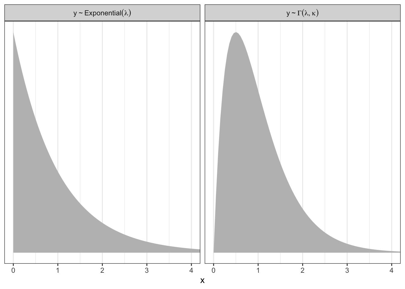
Gamma & Exponential

Code
length_out <- 100

tibble(x = seq(from = 0, to = 5, length.out = length_out)) %>%
  mutate(Gamma       = dgamma(x, 2, 2),

         Exponential = dexp(x)) %>%
  pivot_longer(-x, values_to = "density") %>%
  mutate(label = ifelse(name == "Gamma", "y %~% Gamma(lambda, kappa)", "y %~% Exponential(lambda)")) %>%

  ggplot(aes(x = x, y = density)) +
  geom_area(fill = "grey") +
  #scale_x_continuous(NULL, breaks = NULL) +
  scale_y_continuous(NULL, breaks = NULL) +
  coord_cartesian(xlim = c(0, 4)) +
  theme_bw() +
  facet_wrap(~ label, scales = "free_y", labeller = label_parsed)
Poisson

Code
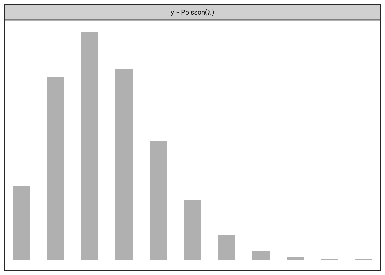
tibble(x = 0:20) %>%
  mutate(density = dpois(x, lambda = 2.5),
         strip   = "y %~% Poisson(lambda)") %>%

  ggplot(aes(x = x, y = density)) +
  geom_col(fill = "grey", width = 1/2) +
  scale_x_continuous(NULL, breaks = NULL) +
  scale_y_continuous(NULL, breaks = NULL) +
  coord_cartesian(xlim = c(0, 10)) +
  theme_bw() +
  facet_wrap(~ strip, labeller = label_parsed)
Binomial

Code
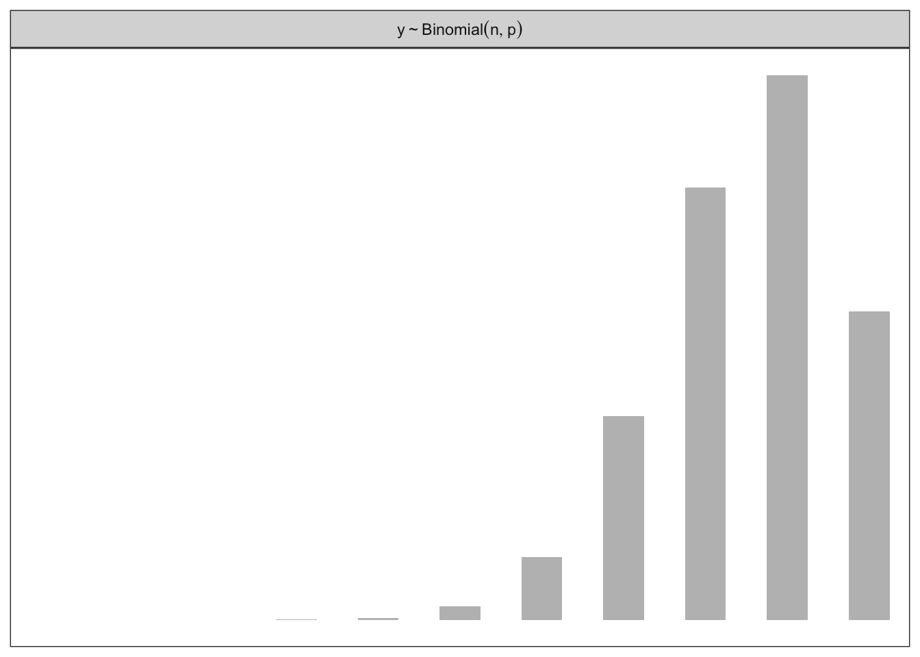
tibble(x = 0:10) %>%
  mutate(density = dbinom(x, size = 10, prob = .85),
         strip   = "y %~% Binomial(n, p)") %>%

  ggplot(aes(x = x, y = density)) +
  geom_col(fill = "grey", width = 1/2) +
  scale_x_continuous(NULL, breaks = NULL) +
  scale_y_continuous(NULL, breaks = NULL) +
  coord_cartesian(xlim = c(0, 10)) +
  theme_bw() +
  facet_wrap(~ strip, labeller = label_parsed)
Slopes & Intercepts

Gaussian

Code
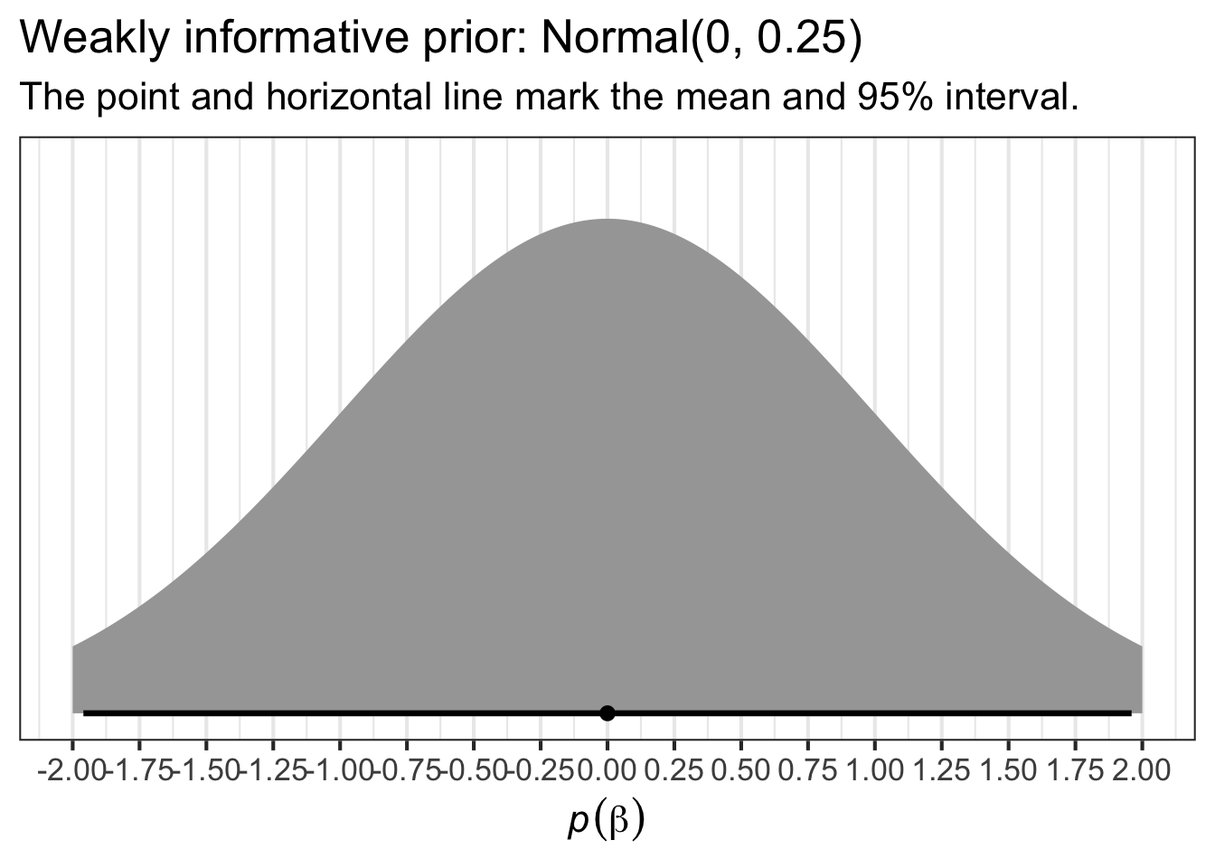
n1 <- prior(normal(0, 1), class = sd) %>%
  parse_dist()

(pn1 <-  ggplot(n1, aes(y = 0, dist = .dist, args = .args)) +
  stat_halfeye(point_interval = mean_qi, .width = .95,
               p_limits = c(.0001, .9999)) +
  scale_y_continuous(NULL, breaks = NULL) +
 scale_x_continuous(breaks = seq(from = -2, to = 2, by = 0.25), limits = c(-2,2))+
  theme_bw(base_size = 16)+
  labs(title = "Weakly informative prior: Normal(0, 0.25)",
       subtitle = "The point and horizontal line mark the mean and 95% interval.",
       x = expression(italic(p)(beta))))
Code
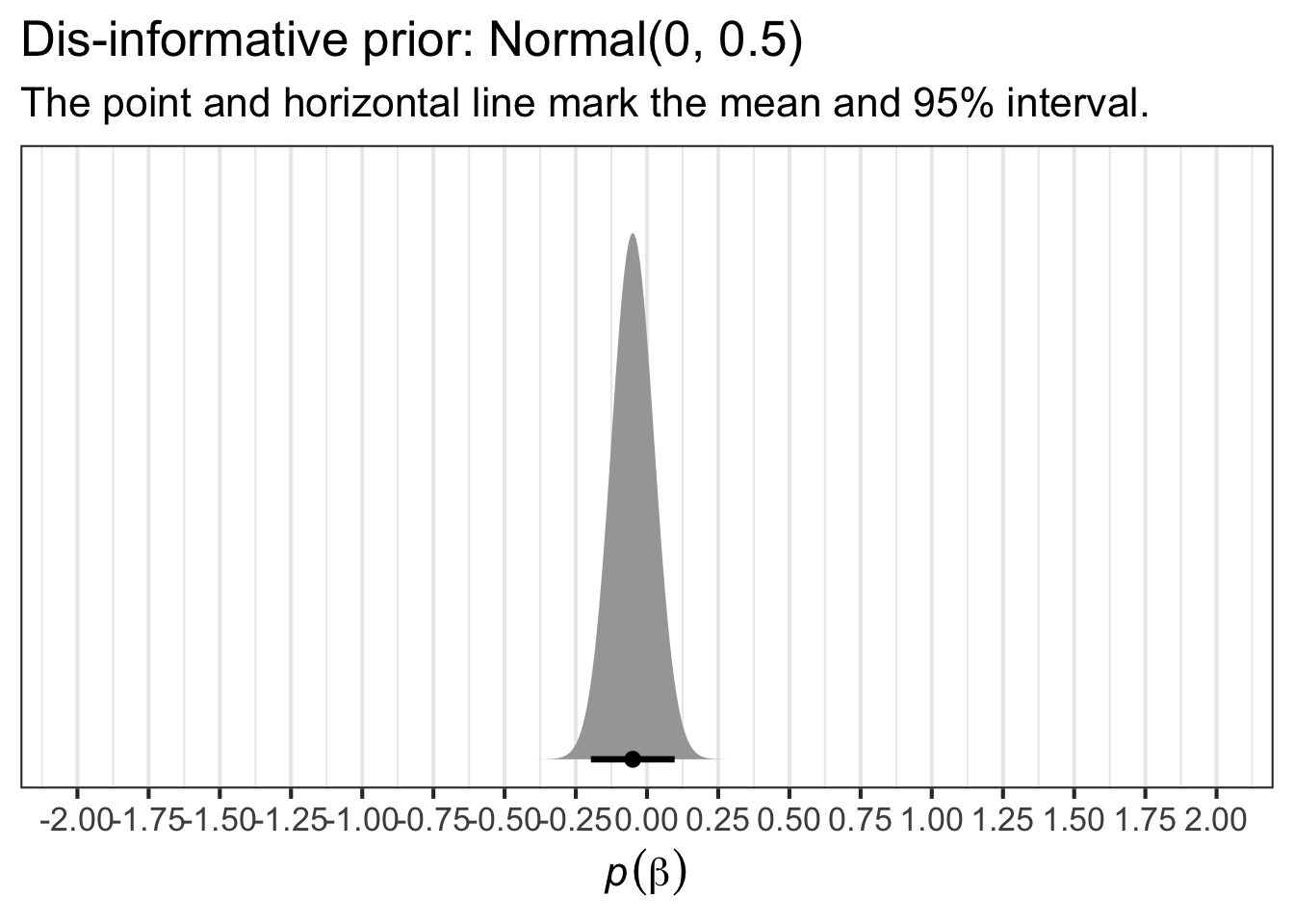
n2 <- prior(normal(-0.05, 0.075), class = sd) %>%
  parse_dist()

(pn2 <- ggplot(n2, aes(y = 0, dist = .dist, args = .args)) +
  stat_halfeye(point_interval = mean_qi, .width = .95,
               p_limits = c(.0001, .9999)) +
  scale_y_continuous(NULL, breaks = NULL) +
 scale_x_continuous(breaks = seq(from = -2, to = 2, by = 0.25), limits = c(-2,2))+
  theme_bw(base_size = 16)+
  labs(title = "Dis-informative prior: Normal(0, 0.5)",
       subtitle = "The point and horizontal line mark the mean and 95% interval.",
       x = expression(italic(p)(beta)))
)
Code
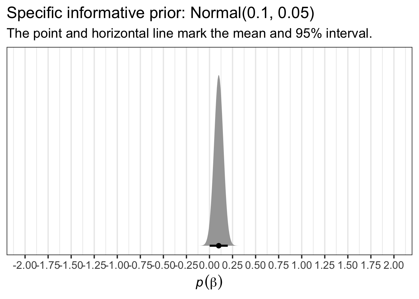
n3 <- prior(normal(0.1, 0.05), class = sd) %>%
  parse_dist()

(pn3 <- ggplot(n3, aes(y = 0, dist = .dist, args = .args)) +
  stat_halfeye(point_interval = mean_qi, .width = .95,
               p_limits = c(.0001, .9999)) +
  scale_y_continuous(NULL, breaks = NULL) +
 scale_x_continuous(breaks = seq(from = -2, to = 2, by = 0.25), limits = c(-2,2))+
  theme_bw(base_size = 16)+
  labs(title = "Specific informative prior: Normal(0.1, 0.05)",
       subtitle = "The point and horizontal line mark the mean and 95% interval.",
       x = expression(italic(p)(beta)))
)
Code
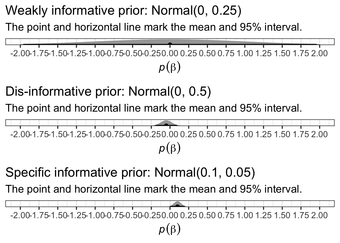
ggpubr::ggarrange(pn1 , pn2, pn3 , nrow  = 3)
Sigma

Sigma is the estimated standard deviation of the errors or, in other words, the standard deviation of the residuals of the model. In the simple case of an intercept-only model, this is identical to the standard deviation of the outcome.

Exponential

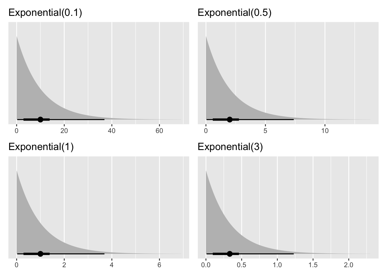
The exponential distribution has a single parameter, \(λ\), which is the reciprocal of the mean.

Code
p0 <- prior(exponential(0.1)) %>%
  ggdist::parse_dist() %>%
  ggplot(aes(y = 0, dist = .dist, args = .args)) +
  ggdist::stat_halfeye(point_interval = mean_qi, .width = c(.5, .95),
               fill = "grey") +
  scale_y_continuous(NULL, breaks = NULL) +
  labs(title = "Exponential(0.1)",
       x = NULL)

p0_5 <- prior(exponential(0.5)) %>%
  ggdist::parse_dist() %>%
  ggplot(aes(y = 0, dist = .dist, args = .args)) +
  ggdist::stat_halfeye(point_interval = mean_qi, .width = c(.5, .95),
               fill = "grey") +
  scale_y_continuous(NULL, breaks = NULL) +
  labs(title = "Exponential(0.5)",
       x = NULL)

p1 <- prior(exponential(1)) %>%
  ggdist::parse_dist() %>%
  ggplot(aes(y = 0, dist = .dist, args = .args)) +
  ggdist::stat_halfeye(point_interval = mean_qi, .width = c(.5, .95),
               fill = "grey") +
  scale_y_continuous(NULL, breaks = NULL) +
  labs(title = "Exponential(1)",
       x = NULL)

p2 <- prior(exponential(3)) %>%
  ggdist::parse_dist() %>%
  ggplot(aes(y = 0, dist = .dist, args = .args)) +
  ggdist::stat_halfeye(point_interval = mean_qi, .width = c(.5, .95),
               fill = "grey") +
  scale_y_continuous(NULL, breaks = NULL) +
  labs(title = "Exponential(3)",
       x = NULL)


p0 + p0_5 +
p1 + p2
Half Cauchy

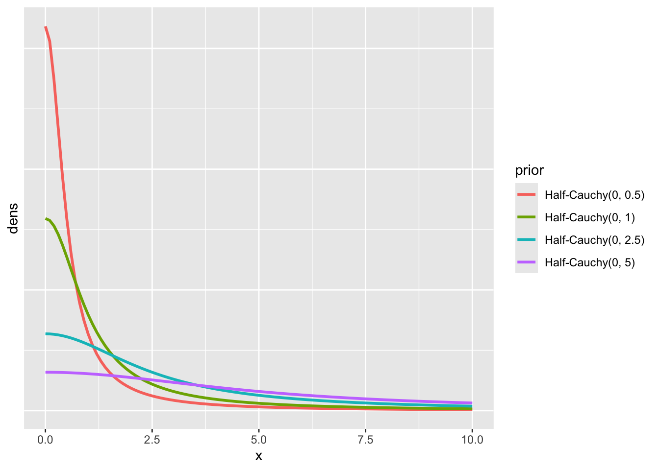
This distribution is helpful for estimating measures like standard deviations. It’s “half” because only the positive values are taken into consideration, since the standard deviation can only ever be positive.

This is how a Half Cauchy distribution with mean 0 and standard deviation 0.1 looks like cauchy(0,0.1):

Code
tibble(scale = c( 0.5, 1, 2.5, 5)) %>%
  crossing(x = seq(0, 10, 0.1)) %>%
  mutate(
    prior = str_c("Half-Cauchy(0, ", scale, ")"),
    dens = dcauchy(x, location = 0, scale = scale)
  ) %>%
  ggplot(aes(x, y = dens)) +
  geom_line(aes(color = prior), linewidth = 1) +
  theme(legend.position.inside = c(0.1, 0.1), axis.ticks.y = element_blank(),axis.text.y = element_blank())
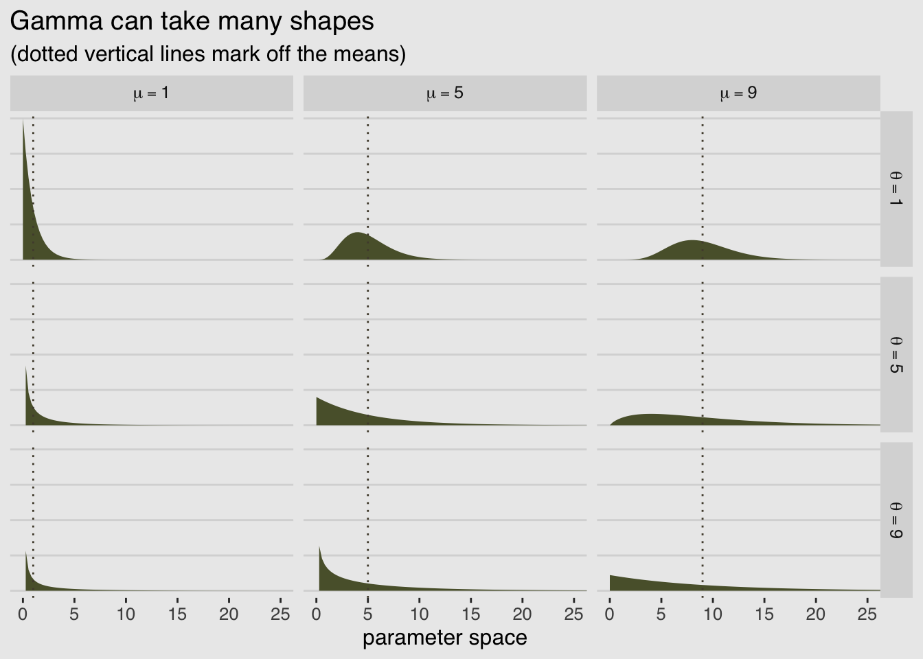
Gamma

Code
library(ggthemes)

# gamma distribution reparametrized by mean (mu) and scale, as in
# McElreath's `rethinking::dgamma2()` (Statistical Rethinking, ch. 10)
dgamma2 <- function(x, mu, scale, log = FALSE) {
  dgamma(x, shape = mu / scale, scale = scale, log = log)
}

# data
crossing(mu    = c(1, 5, 9),
         theta = c(1, 5, 9)) %>%
  expand_grid(x = seq(from = 0, to = 27, length.out = 100)) %>%
  mutate(density    = dgamma2(x, mu, theta),
         mu_char    = str_c("mu==", mu),
         theta_char = str_c("theta==", theta)) %>%

  # plot
  ggplot() +
  geom_area(aes(x = x, y = density),
            fill = canva_pal("Green fields")(4)[4]) +
  geom_vline(aes(xintercept = mu),
             color = canva_pal("Green fields")(4)[2], linetype = 3) +
  scale_y_continuous(NULL, labels = NULL) +
  labs(title = "Gamma can take many shapes",
       subtitle = "(dotted vertical lines mark off the means)",
       x = "parameter space") +
  coord_cartesian(xlim = c(0, 25)) +
  theme_hc() +
  theme(axis.ticks.y = element_blank(),
        plot.background = element_rect(fill = "grey92")) +
  facet_grid(theta_char~mu_char, labeller = label_parsed)
Compare priors on sigma

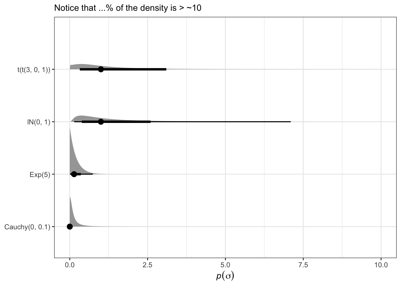
Did you know that if you take the log of a lognormal distribution, you end up with a normal distribution and viceversa? So you should remember: normal priors on log(sigma) are by definition log-normal priors on sigma. The same repeated again: normal prior on the log link is like a lognormal prior on the identity link.

Code
data.frame(sigma = c(exp(dist_normal(0,1)), # exp beacause brms does the log of sigma
                     exp(dist_student_t(3, 0, 1)),
                      dist_cauchy(location = 0, scale = 0.1),
                       dist_exponential(5)
                     )) |>
     ggplot(aes(xdist = sigma,  y = as.character(sigma))) +
     stat_halfeye(p_limits = c(0, 0.975))+
  theme_bw()+
  scale_x_continuous(expression(italic(p)(sigma)), limits = c(0,10))+
  labs(subtitle = "Notice that ...% of the density is > ~10",
       y= NULL)
Code
# Intercept of the delta DOC. remember that in this model the  Intercept is the delta DOC value when the pond water volume assume its average value.
n1 <- prior(normal(0, 5), class = sd) %>%
  parse_dist()

(pn1 <-  ggplot(n1, aes(y = 0, dist = .dist, args = .args)) +
  stat_halfeye(point_interval = mean_qi, .width = .95,
               p_limits = c(.0001, .9999)) +
  scale_y_continuous(NULL, breaks = NULL) +
 scale_x_continuous(breaks = seq(from = -15, to = 15, by = 2.5), limits = c(-15,15))+
  theme_bw(base_size = 16)+
  labs(title = "Intercept prior: Normal(0, 5)",
       subtitle = "The point and horizontal line mark the mean and 95% interval.",
       x = expression(italic(p)(beta[0]))))

# Slope beta_1.How much the pond water volume influence delta DOC.

n2 <- prior(normal(-0.2, 0.25), class = sd) %>%
  parse_dist()

(pn2 <- ggplot(n2, aes(y = 0, dist = .dist, args = .args)) +
  stat_halfeye(point_interval = mean_qi, .width = .95,
               p_limits = c(.0001, .9999)) +
  scale_y_continuous(NULL, breaks = NULL) +
 scale_x_continuous(breaks = seq(from = -1, to = 1, by = 0.25), limits = c(-1,1))+
  theme_bw(base_size = 16)+
  labs(title = "Pond water volume prior: Normal(-0.2, 0.25)",
       subtitle = "There is almost 20% of probability that the slope is > 0",
       x = expression(italic(p)(beta[1])))
)

# What is the probability that beta_1 is > 0 ?
tibble(beta_1 = rnorm(n = 10000, mean = -0.2, sd = 0.25))  |>
  count(beta_1 > 0) |>
  mutate(percent = 100 * n / sum(n))

#### Student-t scale parameter #####

n3 <- prior(lognormal(0, 1), class = sd) %>%
  parse_dist()

(pn3 <- ggplot(n3, aes(y = 0, dist = .dist, args = .args)) +
  stat_halfeye(point_interval = mean_qi, .width = .95,
               p_limits = c(.0001, .9999)) +
  scale_y_continuous(NULL, breaks = NULL) +
  theme_bw(base_size = 16)+
  labs(title = "Student-t scale parameter prior: Normal(0, 1)",
       x = expression(italic(p)(s)))
)

### Student-t nu parameter #####
n4 <- prior(gamma(2, 1)) %>%
  parse_dist()

(pn4 <- ggplot(n4, aes(y = 0, dist = .dist, args = .args)) +
  stat_halfeye(point_interval = mean_qi, .width = .95,
               p_limits = c(.0001, .9999)) +
  scale_y_continuous(NULL, breaks = NULL) +
 scale_x_continuous(breaks = seq(from = 0, to = 9, by = 1.5), limits= c(0,9))+
  theme_bw(base_size = 16)+
  labs(title = "Student-t nu parameter prior: Gamma(2, 1)",
       x = expression(italic(p)(s)))
)

#### merge the plots ####
ggpubr::ggarrange(pn1 , pn2, pn3 , pn4, nrow  = 4)
Back to top
Ecopath with Ecosim (Rpath)
Measurement Error
Source Code
---
title: "Visualize priors"
author: "Leonardo Capitani"
date: "07/17/2026"
date-modified: last-modified
execute:
  echo: true
  warning: false
  message: false
format:
      html:
          toc: true
          code-fold: true
          code-tools: true
          code-link: true
          embed-resources: true
editor: visual
editor_options:
  chunk_output_type: console
---

## Load packages

```{r load_packages}
library(ggdist)
library(distributional)
library(tidyverse)
library(kableExtra)
library(brms)
library(patchwork)
```

## Chapter 10, Statistical rethinking

> One strategy for choosing an outcome distribution is to plot the histogram of the outcome variable and, by gazing into its soul, decide what sort of distribution function to use. Call this strategy **Histomancy**, the ancient art of divining likelihood functions from empirical histograms. This sorcery is used, for example, when testing for normality before deciding whether or not to use a non-parametric procedure. **Histomancy** is a false god. (p. 314, emphasis in the original)
>
> Luckily, it’s easy to do better. By using all of our prior knowledge about the outcome variable, usually in the form of constraints on the possible values it can take, we can appeal to maximum entropy for the choice of distribution. Then all we have to do is generalize the linear regression strategy–replace a parameter describing the shape of the likelihood with a linear model–to probability distributions other than the Gaussian. (p. 313)

## Rethinking: A likelihood is a prior.

> In traditional statistics, likelihood functions are “objective” and prior distributions “subjective.” In Bayesian statistics, likelihoods are deeply related to prior probability distributions: They are priors for the data, conditional on the parameters. And just like with other priors, there is no correct likelihood. But there are better and worse likelihoods, depending upon the context. (McElreath, R. 2020, *Statistical Rethinking*, p. 316).

## Play with distributions

<https://michael-franke.github.io/intro-data-analysis/selected-continuous-distributions-of-random-variables.html>

## Gamma & Exponential

```{r gamma_exponential}
length_out <- 100

tibble(x = seq(from = 0, to = 5, length.out = length_out)) %>%
  mutate(Gamma       = dgamma(x, 2, 2),

         Exponential = dexp(x)) %>%
  pivot_longer(-x, values_to = "density") %>%
  mutate(label = ifelse(name == "Gamma", "y %~% Gamma(lambda, kappa)", "y %~% Exponential(lambda)")) %>%

  ggplot(aes(x = x, y = density)) +
  geom_area(fill = "grey") +
  #scale_x_continuous(NULL, breaks = NULL) +
  scale_y_continuous(NULL, breaks = NULL) +
  coord_cartesian(xlim = c(0, 4)) +
  theme_bw() +
  facet_wrap(~ label, scales = "free_y", labeller = label_parsed)
```

## Poisson

```{r poisson}

tibble(x = 0:20) %>%
  mutate(density = dpois(x, lambda = 2.5),
         strip   = "y %~% Poisson(lambda)") %>%

  ggplot(aes(x = x, y = density)) +
  geom_col(fill = "grey", width = 1/2) +
  scale_x_continuous(NULL, breaks = NULL) +
  scale_y_continuous(NULL, breaks = NULL) +
  coord_cartesian(xlim = c(0, 10)) +
  theme_bw() +
  facet_wrap(~ strip, labeller = label_parsed)
```

## Binomial

```{r binomial}
tibble(x = 0:10) %>%
  mutate(density = dbinom(x, size = 10, prob = .85),
         strip   = "y %~% Binomial(n, p)") %>%

  ggplot(aes(x = x, y = density)) +
  geom_col(fill = "grey", width = 1/2) +
  scale_x_continuous(NULL, breaks = NULL) +
  scale_y_continuous(NULL, breaks = NULL) +
  coord_cartesian(xlim = c(0, 10)) +
  theme_bw() +
  facet_wrap(~ strip, labeller = label_parsed)
```

## Slopes & Intercepts

### Gaussian

```{r gaussian_priors}

n1 <- prior(normal(0, 1), class = sd) %>%
  parse_dist()

(pn1 <-  ggplot(n1, aes(y = 0, dist = .dist, args = .args)) +
  stat_halfeye(point_interval = mean_qi, .width = .95,
               p_limits = c(.0001, .9999)) +
  scale_y_continuous(NULL, breaks = NULL) +
 scale_x_continuous(breaks = seq(from = -2, to = 2, by = 0.25), limits = c(-2,2))+
  theme_bw(base_size = 16)+
  labs(title = "Weakly informative prior: Normal(0, 0.25)",
       subtitle = "The point and horizontal line mark the mean and 95% interval.",
       x = expression(italic(p)(beta))))

n2 <- prior(normal(-0.05, 0.075), class = sd) %>%
  parse_dist()

(pn2 <- ggplot(n2, aes(y = 0, dist = .dist, args = .args)) +
  stat_halfeye(point_interval = mean_qi, .width = .95,
               p_limits = c(.0001, .9999)) +
  scale_y_continuous(NULL, breaks = NULL) +
 scale_x_continuous(breaks = seq(from = -2, to = 2, by = 0.25), limits = c(-2,2))+
  theme_bw(base_size = 16)+
  labs(title = "Dis-informative prior: Normal(0, 0.5)",
       subtitle = "The point and horizontal line mark the mean and 95% interval.",
       x = expression(italic(p)(beta)))
)


n3 <- prior(normal(0.1, 0.05), class = sd) %>%
  parse_dist()

(pn3 <- ggplot(n3, aes(y = 0, dist = .dist, args = .args)) +
  stat_halfeye(point_interval = mean_qi, .width = .95,
               p_limits = c(.0001, .9999)) +
  scale_y_continuous(NULL, breaks = NULL) +
 scale_x_continuous(breaks = seq(from = -2, to = 2, by = 0.25), limits = c(-2,2))+
  theme_bw(base_size = 16)+
  labs(title = "Specific informative prior: Normal(0.1, 0.05)",
       subtitle = "The point and horizontal line mark the mean and 95% interval.",
       x = expression(italic(p)(beta)))
)

ggpubr::ggarrange(pn1 , pn2, pn3 , nrow  = 3)

```

## Sigma

Sigma is the estimated standard deviation of the errors or, in other words, the standard deviation of the residuals of the model. In the simple case of an intercept-only model, this is identical to the standard deviation of the outcome.

### Exponential

The exponential distribution has a single parameter, $λ$, which is the reciprocal of the mean.

```{r exponential_sigma_prior}

p0 <- prior(exponential(0.1)) %>%
  ggdist::parse_dist() %>%
  ggplot(aes(y = 0, dist = .dist, args = .args)) +
  ggdist::stat_halfeye(point_interval = mean_qi, .width = c(.5, .95),
               fill = "grey") +
  scale_y_continuous(NULL, breaks = NULL) +
  labs(title = "Exponential(0.1)",
       x = NULL)

p0_5 <- prior(exponential(0.5)) %>%
  ggdist::parse_dist() %>%
  ggplot(aes(y = 0, dist = .dist, args = .args)) +
  ggdist::stat_halfeye(point_interval = mean_qi, .width = c(.5, .95),
               fill = "grey") +
  scale_y_continuous(NULL, breaks = NULL) +
  labs(title = "Exponential(0.5)",
       x = NULL)

p1 <- prior(exponential(1)) %>%
  ggdist::parse_dist() %>%
  ggplot(aes(y = 0, dist = .dist, args = .args)) +
  ggdist::stat_halfeye(point_interval = mean_qi, .width = c(.5, .95),
               fill = "grey") +
  scale_y_continuous(NULL, breaks = NULL) +
  labs(title = "Exponential(1)",
       x = NULL)

p2 <- prior(exponential(3)) %>%
  ggdist::parse_dist() %>%
  ggplot(aes(y = 0, dist = .dist, args = .args)) +
  ggdist::stat_halfeye(point_interval = mean_qi, .width = c(.5, .95),
               fill = "grey") +
  scale_y_continuous(NULL, breaks = NULL) +
  labs(title = "Exponential(3)",
       x = NULL)


p0 + p0_5 +
p1 + p2
```

#### Half Cauchy

This distribution is helpful for estimating measures like standard deviations. It’s “half” because only the positive values are taken into consideration, since the standard deviation can only ever be positive.

This is how a Half Cauchy distribution with mean 0 and standard deviation 0.1 looks like `cauchy(0,0.1)`:

```{r half_cauchy_plot}
tibble(scale = c( 0.5, 1, 2.5, 5)) %>%
  crossing(x = seq(0, 10, 0.1)) %>%
  mutate(
    prior = str_c("Half-Cauchy(0, ", scale, ")"),
    dens = dcauchy(x, location = 0, scale = scale)
  ) %>%
  ggplot(aes(x, y = dens)) +
  geom_line(aes(color = prior), linewidth = 1) +
  theme(legend.position.inside = c(0.1, 0.1), axis.ticks.y = element_blank(),axis.text.y = element_blank())
```

### Gamma

```{r gamma_prior}
library(ggthemes)

# gamma distribution reparametrized by mean (mu) and scale, as in
# McElreath's `rethinking::dgamma2()` (Statistical Rethinking, ch. 10)
dgamma2 <- function(x, mu, scale, log = FALSE) {
  dgamma(x, shape = mu / scale, scale = scale, log = log)
}

# data
crossing(mu    = c(1, 5, 9),
         theta = c(1, 5, 9)) %>%
  expand_grid(x = seq(from = 0, to = 27, length.out = 100)) %>%
  mutate(density    = dgamma2(x, mu, theta),
         mu_char    = str_c("mu==", mu),
         theta_char = str_c("theta==", theta)) %>%

  # plot
  ggplot() +
  geom_area(aes(x = x, y = density),
            fill = canva_pal("Green fields")(4)[4]) +
  geom_vline(aes(xintercept = mu),
             color = canva_pal("Green fields")(4)[2], linetype = 3) +
  scale_y_continuous(NULL, labels = NULL) +
  labs(title = "Gamma can take many shapes",
       subtitle = "(dotted vertical lines mark off the means)",
       x = "parameter space") +
  coord_cartesian(xlim = c(0, 25)) +
  theme_hc() +
  theme(axis.ticks.y = element_blank(),
        plot.background = element_rect(fill = "grey92")) +
  facet_grid(theta_char~mu_char, labeller = label_parsed)
```

## Compare priors on sigma

::: {.callout-important appearance="simple"}
Did you know that if you take the log of a lognormal distribution, you end up with a normal distribution and viceversa? So you should remember: normal priors on log(`sigma`) are by definition log-normal priors on `sigma`. The same repeated again: normal prior on the log link is like a lognormal prior on the identity link.
:::

```{r}
data.frame(sigma = c(exp(dist_normal(0,1)), # exp beacause brms does the log of sigma
                     exp(dist_student_t(3, 0, 1)),
                      dist_cauchy(location = 0, scale = 0.1),
                       dist_exponential(5)
                     )) |>
     ggplot(aes(xdist = sigma,  y = as.character(sigma))) +
     stat_halfeye(p_limits = c(0, 0.975))+
  theme_bw()+
  scale_x_continuous(expression(italic(p)(sigma)), limits = c(0,10))+
  labs(subtitle = "Notice that ...% of the density is > ~10",
       y= NULL)
```

```{r visualize_priors, eval=FALSE}

# Intercept of the delta DOC. remember that in this model the  Intercept is the delta DOC value when the pond water volume assume its average value.
n1 <- prior(normal(0, 5), class = sd) %>%
  parse_dist()

(pn1 <-  ggplot(n1, aes(y = 0, dist = .dist, args = .args)) +
  stat_halfeye(point_interval = mean_qi, .width = .95,
               p_limits = c(.0001, .9999)) +
  scale_y_continuous(NULL, breaks = NULL) +
 scale_x_continuous(breaks = seq(from = -15, to = 15, by = 2.5), limits = c(-15,15))+
  theme_bw(base_size = 16)+
  labs(title = "Intercept prior: Normal(0, 5)",
       subtitle = "The point and horizontal line mark the mean and 95% interval.",
       x = expression(italic(p)(beta[0]))))

# Slope beta_1.How much the pond water volume influence delta DOC.

n2 <- prior(normal(-0.2, 0.25), class = sd) %>%
  parse_dist()

(pn2 <- ggplot(n2, aes(y = 0, dist = .dist, args = .args)) +
  stat_halfeye(point_interval = mean_qi, .width = .95,
               p_limits = c(.0001, .9999)) +
  scale_y_continuous(NULL, breaks = NULL) +
 scale_x_continuous(breaks = seq(from = -1, to = 1, by = 0.25), limits = c(-1,1))+
  theme_bw(base_size = 16)+
  labs(title = "Pond water volume prior: Normal(-0.2, 0.25)",
       subtitle = "There is almost 20% of probability that the slope is > 0",
       x = expression(italic(p)(beta[1])))
)

# What is the probability that beta_1 is > 0 ?
tibble(beta_1 = rnorm(n = 10000, mean = -0.2, sd = 0.25))  |>
  count(beta_1 > 0) |>
  mutate(percent = 100 * n / sum(n))

#### Student-t scale parameter #####

n3 <- prior(lognormal(0, 1), class = sd) %>%
  parse_dist()

(pn3 <- ggplot(n3, aes(y = 0, dist = .dist, args = .args)) +
  stat_halfeye(point_interval = mean_qi, .width = .95,
               p_limits = c(.0001, .9999)) +
  scale_y_continuous(NULL, breaks = NULL) +
  theme_bw(base_size = 16)+
  labs(title = "Student-t scale parameter prior: Normal(0, 1)",
       x = expression(italic(p)(s)))
)

### Student-t nu parameter #####
n4 <- prior(gamma(2, 1)) %>%
  parse_dist()

(pn4 <- ggplot(n4, aes(y = 0, dist = .dist, args = .args)) +
  stat_halfeye(point_interval = mean_qi, .width = .95,
               p_limits = c(.0001, .9999)) +
  scale_y_continuous(NULL, breaks = NULL) +
 scale_x_continuous(breaks = seq(from = 0, to = 9, by = 1.5), limits= c(0,9))+
  theme_bw(base_size = 16)+
  labs(title = "Student-t nu parameter prior: Gamma(2, 1)",
       x = expression(italic(p)(s)))
)

#### merge the plots ####
ggpubr::ggarrange(pn1 , pn2, pn3 , pn4, nrow  = 4)
```

This website is licensed under a Creative Commons Attributions 4.0 International License


This website is built with and Quarto