Error measurament simulations

library(brms)
library(tidybayes)
library(tidyverse)
library(ggpubr)

# Make random things reproducible
set.seed(1234)

# Bayes stuff
# Use the cmdstanr backend for Stan because it's faster and more modern than
# the default rstan. You need to install the cmdstanr package first
# (https://mc-stan.org/cmdstanr/) and then run cmdstanr::install_cmdstan() to
# install cmdstan on your computer.
options(mc.cores = 4,  # Use 4 cores
        brms.backend = "cmdstanr")
bayes_seed <- 1234

# Colors from MetBrewer
clrs <- MetBrewer::met.brewer("Java")

# Custom ggplot themes to make pretty plots
# Get Roboto Condensed at https://fonts.google.com/specimen/Roboto+Condensed
# Get Roboto Mono at https://fonts.google.com/specimen/Roboto+Mono
theme_pred <- function() {
  theme_minimal(base_family = "Roboto Condensed") +
    theme(panel.grid.minor = element_blank(),
          plot.background = element_rect(fill = "white", color = NA),
          plot.title = element_text(face = "bold"),
          strip.text = element_text(face = "bold"),
          strip.background = element_rect(fill = "grey80", color = NA),
          axis.title.x = element_text(hjust = 0),
          axis.title.y = element_text(hjust = 0),
          legend.title = element_text(face = "bold"))
}

theme_pred_dist <- function() {
  theme_pred() +
    theme(plot.title = element_markdown(family = "Roboto Condensed", face = "plain"),
          plot.subtitle = element_text(family = "Roboto Mono", size = rel(0.9), hjust = 0),
          axis.text.y = element_blank(),
          panel.grid.major.y = element_blank(),
          panel.grid.minor.y = element_blank())
}

theme_pred_range <- function() {
  theme_pred() +
    theme(plot.title = element_markdown(family = "Roboto Condensed", face = "plain"),
          plot.subtitle = element_text(family = "Roboto Mono", size = rel(0.9), hjust = 0),
          panel.grid.minor.y = element_blank())
}

update_geom_defaults("text", list(family = "Roboto Condensed", lineheight = 1))

Introduction

From Gelman et al. 2020 Regression and other stories, p. 458 and Gelman’s blog post on 14.04.2024:

Another form of incomplete data is measurement error. In the linear regression \(y = a+bx+error\), measurement error in \(y\) does not pose a problem, as it folds right into the error term. Suppose we would like to estimate the “underlying” model \(y_i = a + bx_i + e_i\) but \(y\) is itself measured with error, so that what we actually observe is \(y_i^* = y_i + \eta_i\). In that case, we can combine the two models to get \(y_i^* = a + bx_i + e_i + \eta_i\), and if the two error terms are independent and each with mean 0, this reduces to a linear regression of \(y^*\) on \(x\), which can be fit directly. So as long as \(e_i\) is independent of \(\eta_i\) , you can just combine them into a single error term.

Simulate

First , we are going to generate fake data, following the linear relationship \(y_i = a + bx_i + e_i\) with a priori fixed parameters values:

#simulation for measurement error

set.seed(123)

n <- 1000 # number of observations

x <- runif(n, 0, 10) # predictor x with mean = 0 and sd = 10

a <- 0.2 # intercept, the mean value when x = 0
b <- 0.3 # influence of x on y
sigma <- 0.5 # also call in our model "e". It represents to what extent our model is able to predict y.

y <- rnorm(n, a + b*x, sigma)

fake <- data.frame(x,y)

Then fit the linear model \(y_i = a + bx_i + e_i\) to the fake data:

get_prior(formula = y ~ 1 + x, data = fake )

                  prior     class coef group resp dpar nlpar lb ub tag
 student_t(3, 1.7, 2.5) Intercept                                     
                 (flat)         b                                     
                 (flat)         b    x                                
   student_t(3, 0, 2.5)     sigma                             0       
       source
      default
      default
 (vectorized)
      default

fit_1 <- brm(formula = y ~ 1 + x,
             family = gaussian,
             data = fake,
                prior = c(prior(normal(0, 0.2), class = Intercept),
                prior(normal(0, 0.5), class = b),
                prior(exponential(1), class = sigma)),
             iter = 2000, warmup = 1000, cores = 4, chains = 4,
             backend = 'cmdstanr',
             silent = 2, refresh = 0,
      seed = 15)

print(fit_1)

 Family: gaussian 
  Links: mu = identity 
Formula: y ~ 1 + x 
   Data: fake (Number of observations: 1000) 
  Draws: 4 chains, each with iter = 2000; warmup = 1000; thin = 1;
         total post-warmup draws = 4000

Regression Coefficients:
          Estimate Est.Error l-95% CI u-95% CI Rhat Bulk_ESS Tail_ESS
Intercept     0.21      0.03     0.15     0.27 1.00     4485     2994
x             0.30      0.01     0.29     0.31 1.00     4779     3011

Further Distributional Parameters:
      Estimate Est.Error l-95% CI u-95% CI Rhat Bulk_ESS Tail_ESS
sigma     0.50      0.01     0.48     0.52 1.00     3483     3003

Draws were sampled using sample(hmc). For each parameter, Bulk_ESS
and Tail_ESS are effective sample size measures, and Rhat is the potential
scale reduction factor on split chains (at convergence, Rhat = 1).

# generate posterior predictions
pred_1 <- fit_1 |>
  add_predicted_draws(newdata = fake, ndraws = 100,
                  seed = 12345) |> mutate(model = "No Measurement error")

Note

Take home message:

The model returns exactly the fixed values we have previously determined.

Then we are going to add the error measurement \(\eta\) on \(y\) , so \(y_i^* = y_i + \eta_i\). We fixed de measurement error as \(\eta = 1\). Remember that \(e = 0.5\).

sigma_y <- 1
fake$y_star <- rnorm(n, fake$y, sigma_y)

Then we add some error measurement on x, generated \(x^*\). We fixed de measurement error as \(\tau = 4\).

sigma_x <- 4
fake$x_star <- rnorm(n, fake$x, sigma_x)

Then we fit again the same model, but with error measurement on \(y\)

get_prior(formula = y_star ~ 1 + x, data = fake )

                  prior     class coef group resp dpar nlpar lb ub tag
 student_t(3, 1.7, 2.5) Intercept                                     
                 (flat)         b                                     
                 (flat)         b    x                                
   student_t(3, 0, 2.5)     sigma                             0       
       source
      default
      default
 (vectorized)
      default

fit_2 <- brm(formula = y_star ~ 1 + x,
             family = gaussian,
             data = fake,
                prior = c(prior(normal(0, 0.2), class = Intercept),
                prior(normal(0, 0.5), class = b),
                prior(exponential(1), class = sigma)),
             iter = 2000, warmup = 1000, cores = 4, chains = 4,
             backend = 'cmdstanr',
             silent = 2, refresh = 0,
      seed = 15)

print(fit_2)

 Family: gaussian 
  Links: mu = identity 
Formula: y_star ~ 1 + x 
   Data: fake (Number of observations: 1000) 
  Draws: 4 chains, each with iter = 2000; warmup = 1000; thin = 1;
         total post-warmup draws = 4000

Regression Coefficients:
          Estimate Est.Error l-95% CI u-95% CI Rhat Bulk_ESS Tail_ESS
Intercept     0.20      0.07     0.07     0.34 1.00     4166     3134
x             0.29      0.01     0.27     0.32 1.00     4080     3035

Further Distributional Parameters:
      Estimate Est.Error l-95% CI u-95% CI Rhat Bulk_ESS Tail_ESS
sigma     1.11      0.02     1.07     1.16 1.00     3660     2569

Draws were sampled using sample(hmc). For each parameter, Bulk_ESS
and Tail_ESS are effective sample size measures, and Rhat is the potential
scale reduction factor on split chains (at convergence, Rhat = 1).

# generate posterior predictions

pred_2 <- fit_2 |>
  add_predicted_draws(newdata = fake, ndraws = 100,
                  seed = 12345) |> mutate(model = "Measurement error in y")

Then we fit again the same model, but with error measurement on \(x\)

fit_3 <- brm(formula = y ~ 1 + x_star,
             family = gaussian,
             data = fake,
                prior = c(prior(normal(0, 0.2), class = Intercept),
                prior(normal(0, 0.5), class = b),
                prior(exponential(1), class = sigma)),
             iter = 2000, warmup = 1000, cores = 4, chains = 4,
             backend = 'cmdstanr',
             silent = 2, refresh = 0,
      seed = 15)

print(fit_3)

 Family: gaussian 
  Links: mu = identity 
Formula: y ~ 1 + x_star 
   Data: fake (Number of observations: 1000) 
  Draws: 4 chains, each with iter = 2000; warmup = 1000; thin = 1;
         total post-warmup draws = 4000

Regression Coefficients:
          Estimate Est.Error l-95% CI u-95% CI Rhat Bulk_ESS Tail_ESS
Intercept     1.15      0.04     1.07     1.22 1.00     4362     3116
x_star        0.10      0.01     0.09     0.11 1.00     6324     3617

Further Distributional Parameters:
      Estimate Est.Error l-95% CI u-95% CI Rhat Bulk_ESS Tail_ESS
sigma     0.84      0.02     0.81     0.88 1.00     4548     3345

Draws were sampled using sample(hmc). For each parameter, Bulk_ESS
and Tail_ESS are effective sample size measures, and Rhat is the potential
scale reduction factor on split chains (at convergence, Rhat = 1).

# generate posterior predictions

pred_3 <- fit_3 |>
  add_predicted_draws(newdata = fake, ndraws = 100,
                  seed = 12345) |> mutate(model = "Measurement error in x")

Then we fit again the same model, but with error measurement on \(x^*\) and \(y^*\).

fit_4 <- brm(formula = y_star ~ 1 + x_star,
             family = gaussian,
             data = fake,
                prior = c(prior(normal(0, 0.2), class = Intercept),
                prior(normal(0, 0.5), class = b),
                prior(exponential(1), class = sigma)),
             iter = 2000, warmup = 1000, cores = 4, chains = 4,
             backend = 'cmdstanr',
             silent = 2, refresh = 0,
      seed = 15)

print(fit_4)

 Family: gaussian 
  Links: mu = identity 
Formula: y_star ~ 1 + x_star 
   Data: fake (Number of observations: 1000) 
  Draws: 4 chains, each with iter = 2000; warmup = 1000; thin = 1;
         total post-warmup draws = 4000

Regression Coefficients:
          Estimate Est.Error l-95% CI u-95% CI Rhat Bulk_ESS Tail_ESS
Intercept     1.11      0.06     0.99     1.22 1.00     3905     2987
x_star        0.11      0.01     0.09     0.12 1.00     4131     2966

Further Distributional Parameters:
      Estimate Est.Error l-95% CI u-95% CI Rhat Bulk_ESS Tail_ESS
sigma     1.29      0.03     1.24     1.35 1.00     4181     2789

Draws were sampled using sample(hmc). For each parameter, Bulk_ESS
and Tail_ESS are effective sample size measures, and Rhat is the potential
scale reduction factor on split chains (at convergence, Rhat = 1).

# generate posterior predictions

pred_4 <- fit_4 |>
  add_predicted_draws(newdata = fake, ndraws = 100,
                  seed = 12345) |> mutate(model = "Measurement error in both x and y")

Merge the four data frames with model’s predictions

merg <-  rbind(pred_1,pred_2,pred_3,pred_4)

Then we plot:

p1 <- ggplot(pred_1, aes(x = x)) +

  stat_lineribbon(aes(y = .prediction), .width = 0.95, color = "red", fill = "#D1D3D5") +
  geom_point(data = fake, aes(y = y), shape = 1, size = 1, alpha = 0.7) +
  scale_x_continuous(limits = c(-10,20), breaks = seq(from = -10, to = 20, by = 2.5))+
  scale_y_continuous(limits = c(-3, 6))+
  labs(x = "x", y = "y", color = NULL, fill = NULL,
       title = "No measurement error") +
  theme_bw(base_size = 16)


p2 <- ggplot(pred_2, aes(x = x)) +

  stat_lineribbon(aes(y = .prediction), .width = 0.95, color = "red", fill = "#D1D3D5") +
  geom_point(data = fake, aes(y = y_star), shape = 1, size = 1, alpha = 0.7) +
  labs(x = "x", y = expression(y^"*"),color = NULL, fill = NULL,
       title = "Measurement error on y") +
  scale_x_continuous(limits = c(-10,20), breaks = seq(from = -10, to = 20, by = 2.5))+
  scale_y_continuous(limits = c(-3, 6))+
  theme_bw(base_size = 16)

p3 <- ggplot(pred_3, aes(x = x_star)) +

  stat_lineribbon(aes(y = .prediction), .width = 0.95, color = "red", fill = "#D1D3D5") +
  geom_point(data = fake, aes(y = y), shape = 1,size = 1, alpha = 0.7) +
  labs(x = expression(x^"*"), y = "y",color = NULL, fill = NULL,
       title = "Measurement error on x") +
  scale_x_continuous(limits = c(-10,20), breaks = seq(from = -10, to = 20, by = 2.5))+
  scale_y_continuous(limits = c(-3, 6))+
  theme_bw(base_size = 16)

p4 <- ggplot(pred_4, aes(x = x_star)) +

  stat_lineribbon(aes(y = .prediction), , color = "red", fill= "#D1D3D5", .width = 0.95) +
  geom_point(data = fake, aes(y = y_star),shape = 1,  size = 1, alpha = 0.7) +
  labs(x = expression(x^"*"), y =expression(y^"*"),color = NULL, fill = NULL,
       title = "Measurement error in both x and y") +
  scale_x_continuous(limits = c(-10,20), breaks = seq(from = -10, to = 20, by = 2.5))+
  scale_y_continuous(limits = c(-3, 6))+
  theme_bw(base_size = 16)


ggarrange(p1, p2, p3, p4,

          ncol = 2, nrow = 2)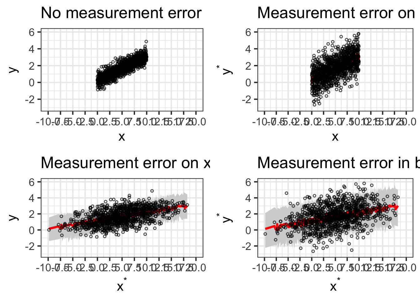

We can compare the regression coefficients:

tidy_inter_1 <-  bayesplot::mcmc_intervals_data(fit_1,
              prob = 0.66, # 66% intervals
              prob_outer = 0.95,#95% intervals
           pars = vars(-contains(c("prior_", "lprior", "lp__")))) |> mutate(model = "No Measurement error")

tidy_inter_2 <-  bayesplot::mcmc_intervals_data(fit_2,
              prob = 0.66, # 66% intervals
              prob_outer = 0.95,#95% intervals
           pars = vars(-contains(c("prior_", "lprior", "lp__")))) |> mutate(model = "Measurement error in y")

tidy_inter_3 <-  bayesplot::mcmc_intervals_data(fit_3,
              prob = 0.66, # 66% intervals
              prob_outer = 0.95,#95% intervals
           pars = vars(-contains(c("prior_", "lprior", "lp__")))) |> mutate(model = "Measurement error in x")

tidy_inter_4 <-  bayesplot::mcmc_intervals_data(fit_4,
              prob = 0.66, # 66% intervals
              prob_outer = 0.95,#95% intervals
           pars = vars(-contains(c("prior_", "lprior", "lp__")))) |> mutate(model = "Measurement error in both x and y")


me <- rbind(tidy_inter_1, tidy_inter_2 , tidy_inter_3, tidy_inter_4) |> filter(parameter != "Intercept")

levels(me$parameter)[levels(me$parameter) == "b_x_star"] <- "b_x" # rename the b parameter where we use x_star

pos <- position_nudge(y = case_when(me$model == "No Measurement error" ~ 0,
                                 me$model  == "Measurement error in y" ~ 0.05,
                                  me$model  == "Measurement error in x" ~ 0.1,
                                    me$model  == "Measurement error in both x and y" ~ 0.15))


ggplot(me, aes(x = m, y = factor(parameter), color = model)) +
   geom_pointinterval(aes(xmin = l, xmax = h), position = pos, size = 8)+
   geom_pointinterval(aes(xmin = ll, xmax = hh), position = pos, size = 2)+
   geom_point( position = pos, color = "black")+
  theme_bw(base_size = 18) +
  scale_color_brewer(palette = "Set1")+
  labs(x = NULL, y = NULL)+
  scale_x_continuous(breaks = seq(from = 0, to = 2, by = 0.15))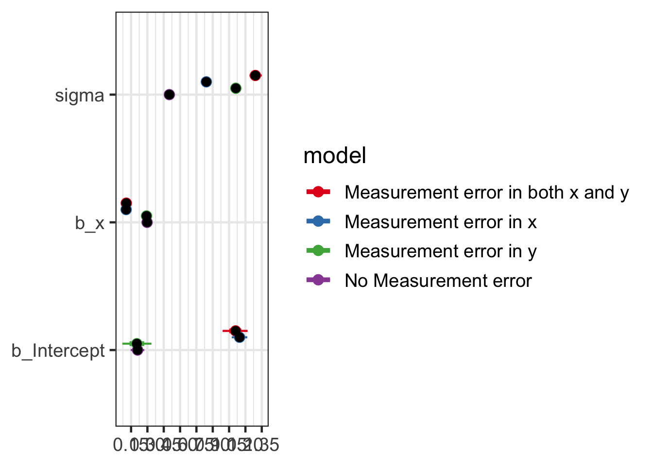

ImportantTake home messages:

The slope \(b\) changes with measurement error in \(x\) but not in \(y\).

When you have measurement error in \(x\), two things happen to attenuate \(b\)—that is, to pull the regression coefficient toward zero.

1. First, if you spreading out \(x\) but keep \(y\) unchanged, this will reduce the slope \(b\) of \(y\) on \(x\).
2. Second, when you add noise to \(x\) you’re changing the ordering of the data, which will reduce the strength of the relationship.

Fitting a Bayesian regression with error measuraments on predictors \(x\)

Please see here.